Bivariate Visualizations
Review: Univariate Viz
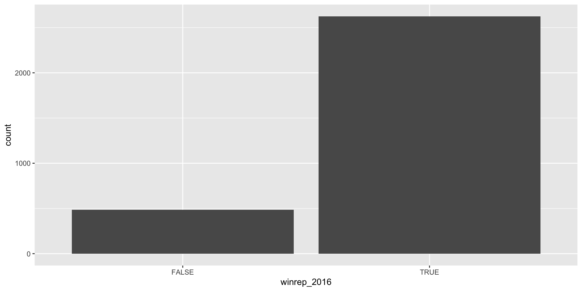
Categorical Variable: Bar Plot
Review: Univariate Viz
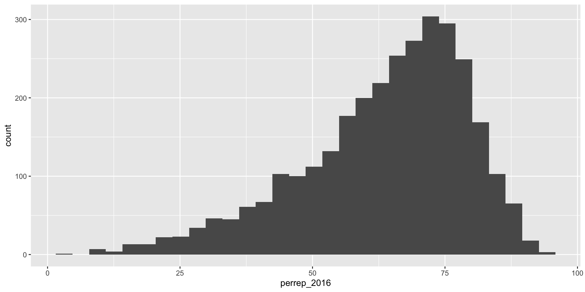
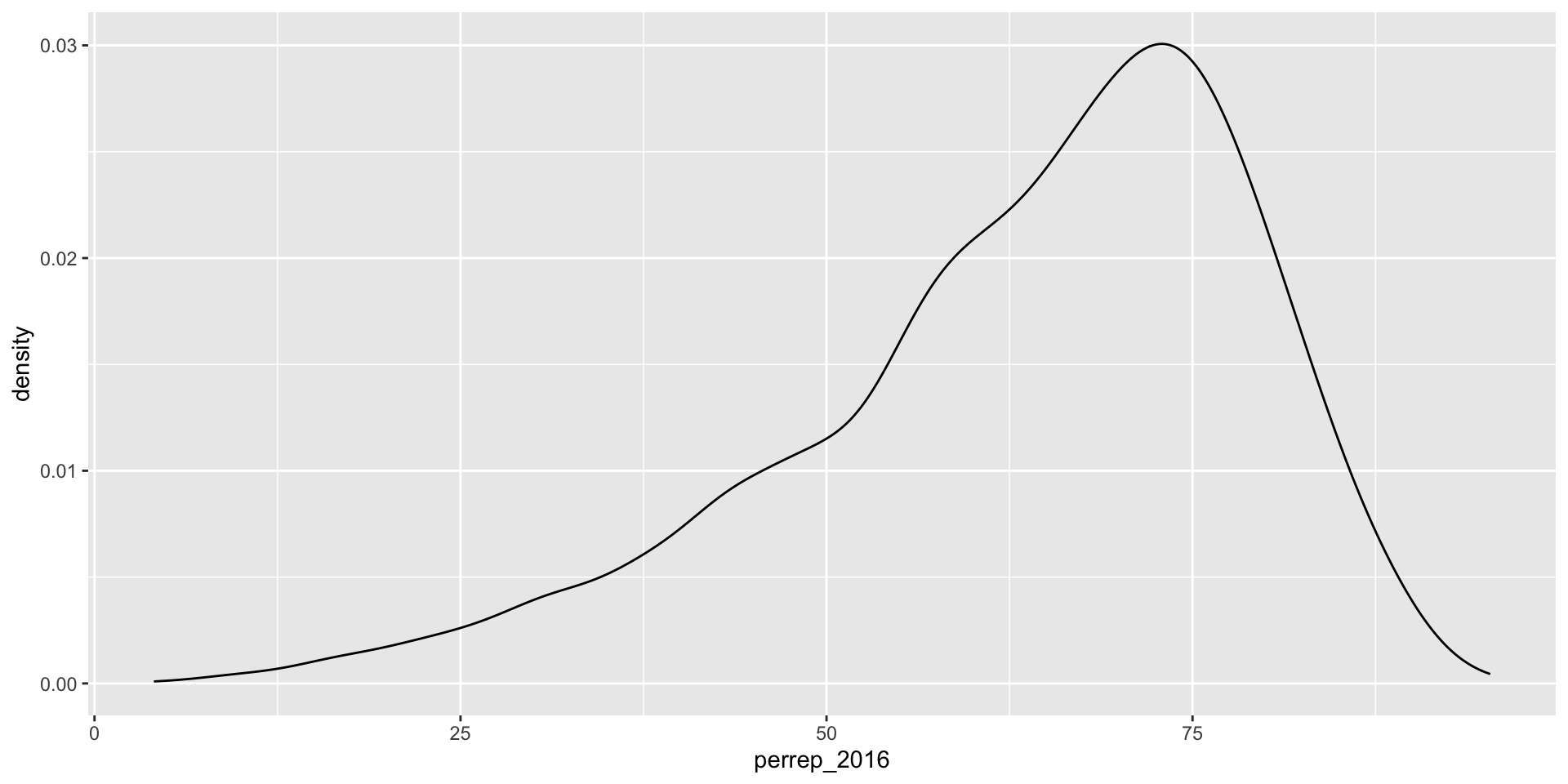
Quantitative Variable: Histogram or Density plot
Preview: Bivariate Viz
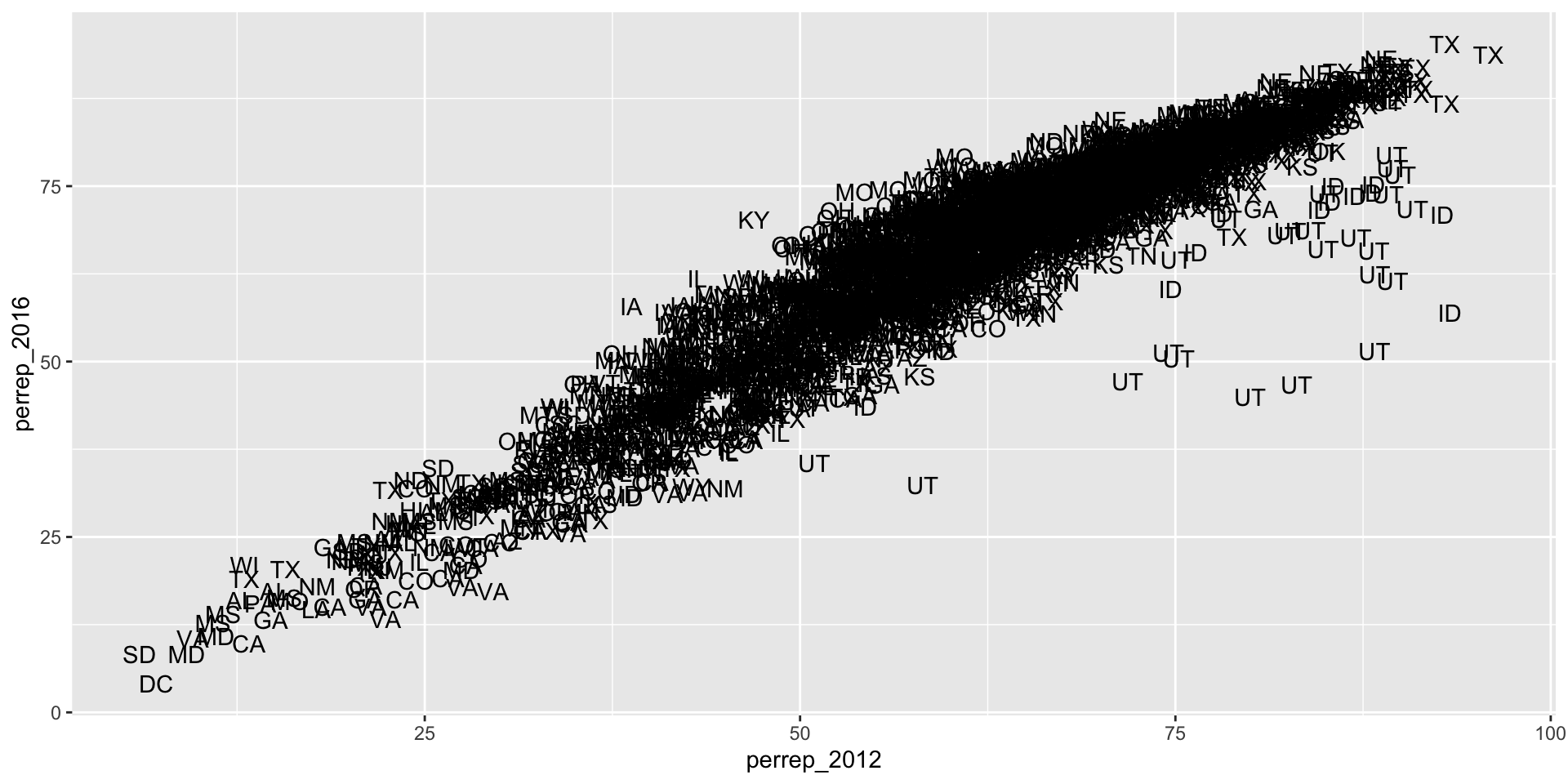
Quantitative + Quantitative Variable: Scatterplot
Preview: Bivariate Viz
Quantitative + Categorical Variable: Density Plots, Boxplots, etc.
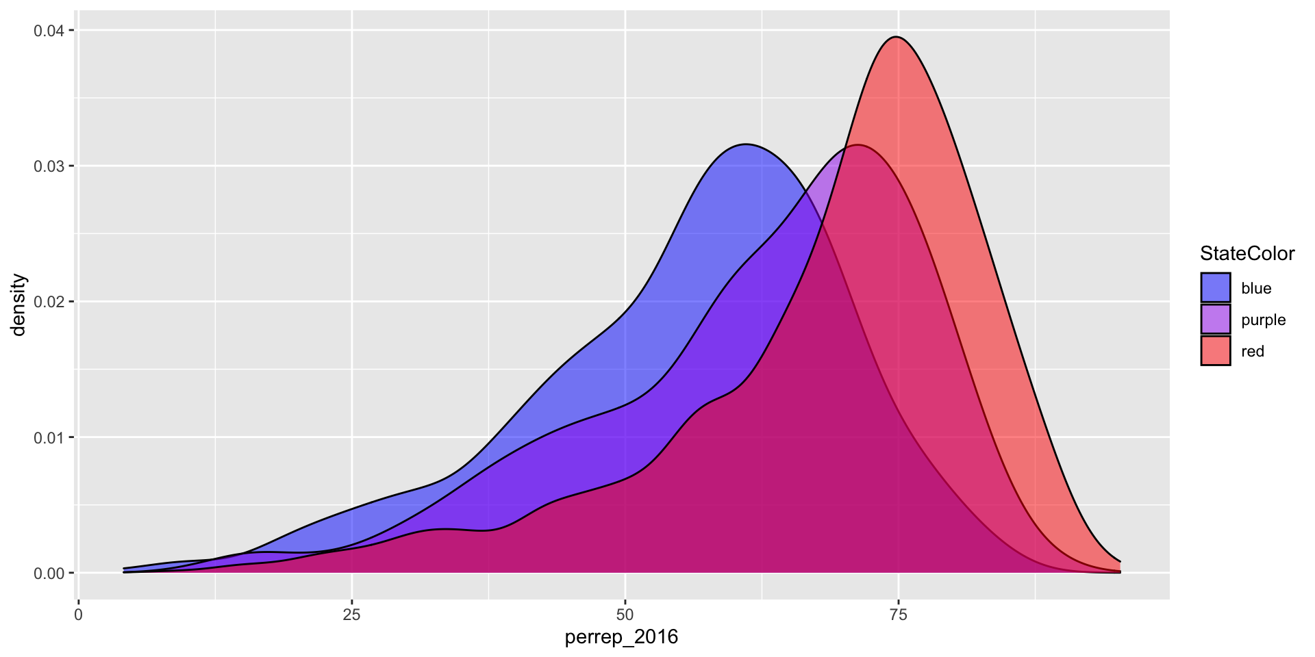
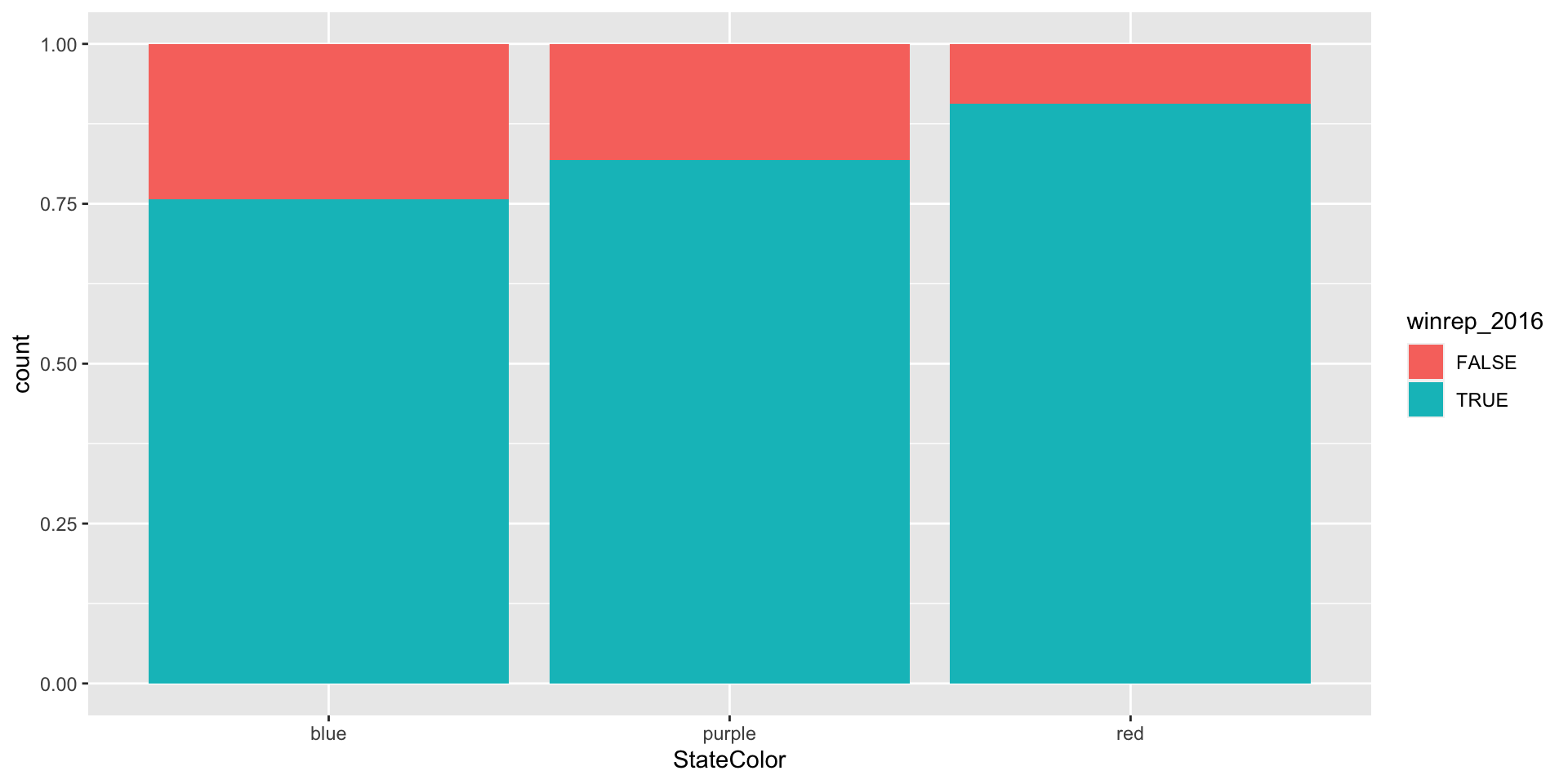
Preview: Bivariate Viz
Categorical + Categorical Variable: side-by-side, proportion Bar plots, etc.
After Class
You’ll make sure to complete Exercise 8-17 (4 of them only require running preexisting code) for the Assignment 3 (due next Tues).
For Friday’s class, meet in the Library (Idea Lab for morning, Lib 206 for FYC)!