Joining Data

Brianna Heggeseth

Announcements

This week in MSCS

Preceptor Training (if you are preceptor for another class!)
Wednesday 3:30pm: Math Problem Solving!
Thursday 11:15am: Coffee Break! Student Advisor Board Introductions!

Due this Week

Assignment 6 (Six Main Verbs) + 7 (Reshaping) on Tuesday [via Moodle]

If you haven’t turned in the following, do so soon:

Tidy Tuesday 4
Iterative Viz 0 (no extra work, submit 1 completed TT html file)
Reflection on Learning (in individual document shared with you)

If your spreadsheet says “No submission for assignment”,

submit your assignment to Moodle
email Brianna indicating that you’ve submitted
Brianna will be going through past assignments Tuesday

Learning Goals

Understand the concept of keys and variables that uniquely identify rows or cases
Understand the different types of joins, different ways of combining two data frames together
Develop comfort in using mutating joins: left_join, inner_join and full_join in the dplyr package
Develop comfort in using filtering joins: semi_join, anti_join in the dplyr package

Template File

Download a template .Rmd of this activity. Put the file in a Day_09 folder within your COMP_STAT_112 folder.

This .Rmd only contains examples that we’ll work on in class and 6 exercises you’ll finish for Assignment 8.

Joins

Definition

A join is a verb that means to combine two data tables.

These tables are often called the left and the right tables.

Left and Right Tables with intersecting light grey lines indicating potential matches and colored points indicating a match.

Kinds of Joins

All joins involve establishing a correspondence — a match — between each case in the left table and zero or more cases in the right table.
The various joins differ in how they handle multiple matches or missing matches.

Matches

Definition of Match

A match between a case in the left data table and a case in the right data table is made based on the values in keys, variables that uniquely define observations in a data table.

Two Types of Keys

A primary key uniquely identifies an observation in its own table.
A foreign key uniquely identifies an observation in another table.

Match in Practice

In order to establish a match between two data tables,

You specify which variables (or keys) to use.
Each variable is specify as a pair, where one variable from the left table corresponds to one variable from the right table.
Cases must have exactly equal values in the left variable and right variable for a match to be made.

Example - Student Grades and Courses

Student grades.
sid	sessionID	grade
S31842	session2207	B+
S32436	session3172	S
S31671	session3435	A-
S31929	session3512	NC

Information about each course section.
sessionID	dept	level	sem	enroll	iid
session2780	O	300	SP2003	21	inst298
session3520	k	300	FA2004	16	inst463
session1965	d	100	FA2001	25	inst414
session3257	o	200	SP2004	16	inst312

Example - Student Grades and Courses

What variables are the primary keys (uniquely identifies a case) for Grades?

sid (student ID) and sessionID (class ID) are the primary keys for Grades as they unique identify each case.

What variables are the primary keys (uniquely identifies a case) for Courses?

sessionID (class ID) and dept are the primary keys for Courses as they unique identify each case. You may have thought that sessionID alone was sufficient; however, if a course is cross-listed, then it may have multiple departments listed.

Example - Student Grades and Courses

What variables are the foreign keys in Grades for Courses?

sessionID (class ID) is part of a foreign key in Grades for Courses. If we group_by and summarize first to deal with cross-listed courses, then sessionID is the foreign key in Grades for Courses.

What variables are the foreign keys in Courses for Grades?

sessionID in Courses is only part of a foreign key that uniquely identify rows in Grades.

Mutating Joins

A mutating join allows you to combine variables from two tables. It first matches observations by their keys, then copies across variables from one table to the other.

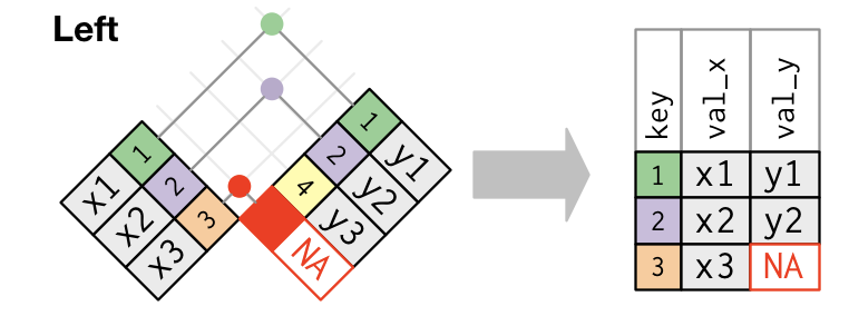
left_join(): the output has all cases from the left, regardless if there is a match in the right, but discards any cases in the right that do not have a match in the left.

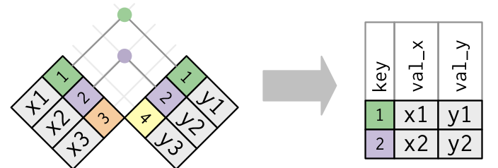
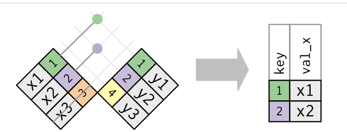
inner_join(): the output has only the cases from the left with a match in the right.

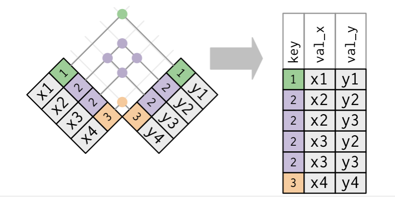
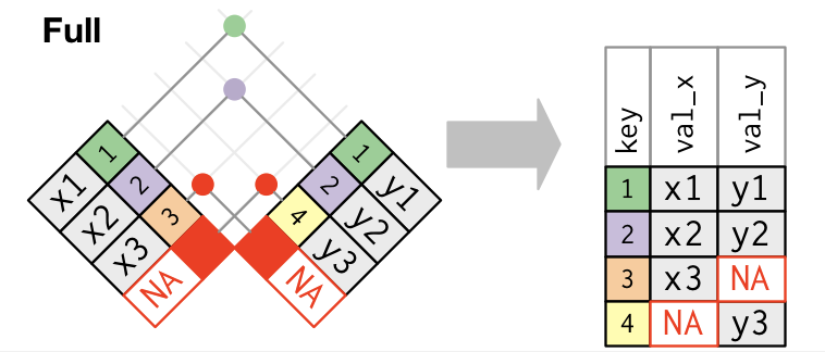
full_join(): the output has all cases from the left and the right. This is less common than the first two join operators.

Example - Student Grades and Courses

Determine the average class size from the viewpoint of the Provost / Admissions Office

How would you approach this?

CourseSizes <- Courses %>%
  group_by(sessionID) %>% # needed for cross-listed courses
  summarise(total_enroll = sum(enroll))

head(CourseSizes)

# A tibble: 6 × 2
  sessionID   total_enroll
  <chr>              <dbl>
1 session1784           22
2 session1785           52
3 session1791           22
4 session1792           20
5 session1794           22
6 session1795           26

mean(CourseSizes$total_enroll)

[1] 21.45251

Example - Student Grades and Courses

Determine the average class size from the viewpoint of a student (average class size for each student experiences across their courses)

How would you approach this?

EnrollmentsWithClassSize <- Grades %>%
  left_join(CourseSizes,
    by = c("sessionID" = "sessionID")
  ) %>%
  select(sid, sessionID, total_enroll)

head(EnrollmentsWithClassSize)

# A tibble: 6 × 3
  sid    sessionID   total_enroll
  <chr>  <chr>              <dbl>
1 S31185 session1784           22
2 S31185 session1785           52
3 S31185 session1791           22
4 S31185 session1792           20
5 S31185 session1794           22
6 S31185 session1795           26

AveClassEachStudent <- EnrollmentsWithClassSize %>%
  group_by(sid) %>%
  summarise(ave_enroll = mean(total_enroll, na.rm = TRUE))

head(AveClassEachStudent)

# A tibble: 6 × 2
  sid    ave_enroll
  <chr>       <dbl>
1 S31185       29  
2 S31188       27.6
3 S31191       29.1
4 S31194       19.5
5 S31197       26.3
6 S31200       26.5

mean(AveClassEachStudent$ave_enroll)

[1] 24.41885

Filtering Joins

Filtering joins affect the observations, not the variables.

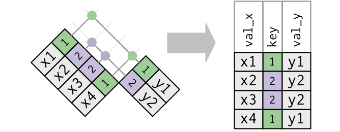
semi_join(): discards any cases in the left table that do not have a match in the right table. If there are multiple matches of right cases to a left case, it keeps just one copy of the left case.

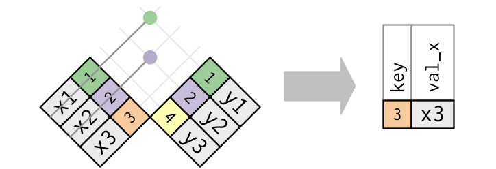
anti_join(): discards any cases in the left table that have a match in the right table.

Example - Student Grades and Courses

Find a subset of the Grades data that only contains data on the four largest sections in the Courses data set.

LargeSections <- Courses %>%
  group_by(sessionID) %>%
  summarise(total_enroll = sum(enroll)) %>%
  arrange(desc(total_enroll)) %>% head(4)

LargeSections

# A tibble: 4 × 2
  sessionID   total_enroll
  <chr>              <dbl>
1 session2956          120
2 session2171          105
3 session2465           93
4 session2170           85

GradesFromLargeSections <- Grades %>%
  semi_join(LargeSections)

head(GradesFromLargeSections)

# A tibble: 6 × 3
  sid    sessionID   grade
  <chr>  <chr>       <chr>
1 S31188 session2956 S    
2 S31344 session2465 S    
3 S31365 session2956 S    
4 S31389 session2170 A-   
5 S31389 session2465 S    
6 S31482 session2170 B+

Example - Student Grades and Courses

Use semi_join() to create a table with a subset of the rows of Grades corresponding to all classes taken in department J.

JCourses <- Courses %>%
  filter(dept == "J")

JGrades <- Grades %>%
  semi_join(JCourses)

After Class

Work on the 6 exercises to turn in for Assignment 8.

These exercises help you deepen your understanding of

Data Wrangling (6 Main Verbs)
Data Visualization (including Spatial Viz)