LASSO

Brianna Heggeseth

As we gather

• Sit with new people today.
  • Introduce yourselves!
  • Share something you would like to learn / be better at.
• Open today’s Rmd in RStudio.
  • Note that I’ve moved the R code reference section to the end of the Rmd, but kept the eval = FALSE chunks. If you don’t like these, you can do a find-and-replace to remove them, but you won’t be able to knit your document right away.

Announcements

• Wednesday at 12-1pm in OLRI 250 - MSCS Talk
• Ethics in Predictive Mental Health Applications: Building Tools to Interrogate our own Stances by Leah Ajmani
• Thursday at 11:15am - MSCS Coffee Break
  • Smail Gallery
• On Thursday, I will assign you groups for ~2.5 weeks
  • If working with someone in class would be a barrier to your learning, let me know.
• Check out this Minnesota Public Radio (MPR) interview on Can AI replace your doctor?! It’s a discussion of AI / machine learning in medicine. NOTE: ML is a subset of AI. (image from Wiki)

• Now that we’re on MPR, journalist David Montgomery used R for data analysis and visualizations using this custom ggtheme to make visuals for MPR. To create a custom ggtheme, check out https://themockup.blog/posts/2020-12-26-creating-and-using-custom-ggplot2-themes/.

Notes - LASSO

CONTEXT

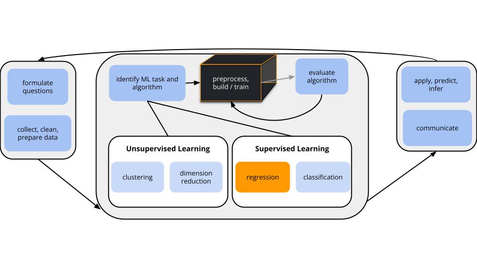
• world = supervised learning
  We want to model some output variable \(y\) using a set of potential predictors \((x_1, x_2, ..., x_p)\).

• task = regression
  \(y\) is quantitative

• model = linear regression
  We’ll assume that the relationship between \(y\) and (\(x_1, x_2, ..., x_p\)) can be represented by

  \[y = \beta_0 + \beta_1 x_1 + \beta_2 x_2 + ... + \beta_p x_p + \varepsilon\]

• estimation algorithm = LASSO (instead of Least Squares)

Notes - LASSO

Least Absolute Shrinkage and Selection Operator

• Dates back to 1996, proposed by Robert Tibshirani (one of the authors of ISLR)

Use the LASSO algorithm to help us regularize and select the “best” predictors \(x\) to use in a predictive linear regression model of \(y\):

\[y = \hat{\beta}_0 + \hat{\beta}_1 x_1 + \cdots + \hat{\beta}_p x_p + \varepsilon\]

Idea

• Penalize a predictor for adding complexity to the model (by penalizing its coefficient).
• Track whether the predictor’s contribution to the model (lowering RSS) is enough to offset this penalty.

Algorithm Criterion

Identify the model coefficients \(\hat{\beta}_1, \hat{\beta}_2, ... \hat{\beta}_p\) that minimize the penalized residual sum of squares:

\[RSS + \lambda \sum_{j=1}^p \vert \hat{\beta}_j\vert = \sum_{i=1}^n (y_i - \hat{y}_i)^2 + \lambda \sum_{j=1}^p \vert \hat{\beta}_j\vert\]

where

• residual sum of squares (RSS) measures the overall model prediction error
• the penalty term measures the overall size of the model coefficients
• \(\lambda \ge 0\) (“lambda”) is a tuning parameter

Small Group Discussion

Discuss basic understanding from the video to help each other clear up concepts.

EXAMPLE 1: LASSO vs other algorithms for building linear regression models

1. LASSO vs least squares
   • What’s one advantage of LASSO vs least squares?
   • Which algorithm(s) require us (or R) to scale the predictors?

2. What is one advantage of LASSO vs backward stepwise selection?

Small Group Discussion

EXAMPLE 2: LASSO tuning

We have to pick a \(\lambda\) penalty tuning parameter for our LASSO model. What’s the impact of \(\lambda\)?

1. When \(\lambda\) is 0, …

2. As \(\lambda\) increases, the predictor coefficients ….

3. Goldilocks problem:

   • If \(\lambda\) is too big, ….
   • If \(\lambda\) is too small, …

4. To decide between a LASSO that uses \(\lambda = 0.01\) vs \(\lambda = 0.1\) (for example), we can ….

Picking \(\lambda\)

We cannot know the “best” value for \(\lambda\) in advance. This varies from analysis to analysis.

We must try a reasonable range of possible values for \(\lambda\). This also varies from analysis to analysis.

In general, we have to use trial-and-error to identify a range that is…

• wide enough that it doesn’t miss the best values for \(\lambda\)
• narrow enough that it focuses on reasonable values for \(\lambda\)

Small Group Activity

Go to https://bcheggeseth.github.io/253_spring_2024/schedule.html

Open Rmd for today.

Go to > Exercises.

• Work on implementing LASSO to familiar data
• Become familiar with the new code structures
  • instead of fit_resamples to run CV, we’ll use tune_grid to tune the algorithm with CV
  • new engine: set_engine('glmnet')
• Ask me questions as I move around the room.

After Class

• Finish the activity, check the solutions, and reach out with questions.
• There’s an R code reference section at the end, and optional R code tutorial videos posted for today’s material.
• If you’re curious, there’s an optional “deeper learning” section below that presents two other shrinkage algorithms that we won’t cover in this course.
• Continue to check in on Slack. I’ll be posting announcements there from now on.

Upcoming due dates

• Nothing due Thursday

• Due next Tuesday:

  • Homework 3 (now posted)
  • Checkpoint 6 (will be posted Thursday)