Evaluating Classification Models

Brianna Heggeseth

As we gather

• Sit where ever you’d like
  • Introduce yourself!
• Open today’s Rmd

Announcements

MSCS Events

• Thursday at 11:15am - MSCS Coffee Break

  • Smail Gallery

• Thursday, March 7, 4:45pm, OLRI 250: Joseph Johnson, “Advertising and Sex Cells: Analogies between the Development of Size Difference in Sex Cells and the Development of Name Brand and Generics”

• Monday, March 25, 4:45pm, JBD: MSCS & Society Lecture

Announcements

Next Group Formation

• Fill out form with preference for next group for Group Assignment 2

Concept Quiz 1

• Revise Quiz 1 Part 1 (due Friday at 5pm)
• I’ll pass them out at the end of class.
• I’m working on Part 2. Feedback will be shared online.

Where are we?

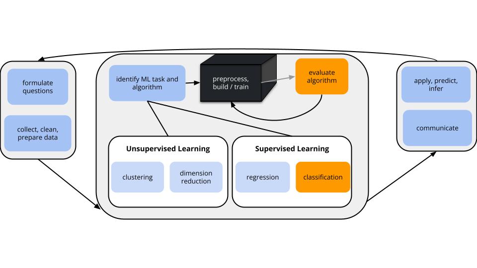
CONTEXT

• world = supervised learning
  We want to model some output variable \(y\) using a set of potential predictors \((x_1, x_2, ..., x_p)\).

• task = CLASSIFICATION
  \(y\) is categorical and binary

• (parametric) algorithm
  logistic regression

• application = classification

  • Use our algorithm to calculate the probability that y = 1.
  • Turn these into binary classifications using a classification rule. For some probability threshold c:
    • If the probability that y = 1 is at least c, classify y as 1.
    • Otherwise, classify y as 0.
  • WE get to pick c. This should be guided by context (what are the consequences of misclassification?) and the quality of the resulting classifications.

GOAL

Evaluate the quality of binary classifications of \(y\) (here resulting logistic regression model).

Notes: Sensitivity and Specificity

\[\begin{split} \text{overall accuracy} & = \text{probability of making a correct classification} \\ \text{sensitivity} & = \text{true positive rate}\\ & = \text{probability of correctly classifying $y=1$ as $y=1$} \\ \text{specificity} & = \text{true negative rate} \\ & = \text{probability of correctly classifying $y=0$ as $y=0$} \\ \text{1 - specificity} & = \text{false positive rate} \\ & = \text{probability of classifying $y=0$ as $y=1$} \\ \end{split}\]

In-sample estimation (how well our model classifies the same data points we used to build it)

	y = 0	y = 1
classify as 0	a	b
classify as 1	c	d

\[\begin{split} \text{overall accuracy} & = \frac{a + d}{a + b + c + d}\\ \text{sensitivity} & = \frac{d}{b + d} \\ \text{specificity} & = \frac{a}{a + c} \\ \end{split}\]

k-Fold Cross-Validation (how well our model classifies NEW data points)

• Divide the data into k folds of approximately equal size.
  
• Repeat the following procedures for each fold j = 1, 2, …, k:
  • Remove fold j from the data set.
    
  • Fit a model using the other k - 1 folds.
    
  • Use this model to classify the outcomes for the data points in fold j.
    
  • Calculate the overall accuracy, sensitivity, and specificity of these classifications.
    
• Average the metrics across the k folds. This gives our CV estimates of overall accuracy, sensitivity, and specificity.

Notes: ROC curves

ROC: Receiver operating characteristic curves

Sensitivity and specificity depend upon the specific probability threshold c.

• If we lower c, hence make it easier to classify y as 1
  • sensitivity increases but specificity decreases
• If we increase c, hence make it tougher to classify y as 1
  • specificity increases but sensitivity decreases

To understand this trade-off, for a range of possible thresholds c between 0 and 1, ROC curves calculate and plot

• y-axis: sensitivity (true positive rate)
• x-axis: 1 - specificity (false positive rate)
  Since specificity is the probability of classifying y = 0 as 0, 1 - specificity is the misclassifying y = 0 as 1.

Why we care:

• Along with context, ROC curves can help us identify an appropriate probability threshold c.
• ROC curves can help us compare the quality of different models.
• The area under an ROC curve (AUC) estimates the probability that our algorithm is more likely to classify y = 1 as 1 than to classify y = 0 as 1, hence distinguish between the 2 classes.

Small Group Discussion

Open up your Rmd file.

Example 1

Suppose we model RainTomorrow in Sydney using only the number of hours of bright Sunshine today.

Using a probability threshold of 0.5, this model produces the following classification rule:

• If Sunshine < 3.125, predict rain.
• Otherwise, predict no rain.

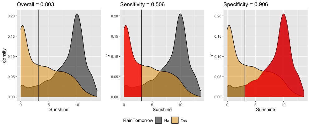
Interpret these in-sample estimates of the resulting classification quality.

1. Overall accuracy = 0.803
   • We correctly predict the rain outcome (yes or no) 80.3% of the time.
   • We correctly predict “no rain” on 80.3% of non-rainy days.
   • We correctly predict “rain” on 80.3% of rainy days.
2. Sensitivity = 0.506
   • We correctly predict the rain outcome (yes or no) 50.6% of the time.
   • We correctly predict “no rain” on 50.6% of non-rainy days.
   • We correctly predict “rain” on 50.6% of rainy days.
3. Specificity = 0.906
   • We correctly predict the rain outcome (yes or no) 90.6% of the time.
   • We correctly predict “no rain” on 90.6% of non-rainy days.
   • We correctly predict “rain” on 90.6% of rainy days.

Example 1

Interpret these in-sample estimates of the resulting classification quality.

1. Overall accuracy = 0.803
   • We correctly predict the rain outcome (yes or no) 80.3% of the time.
2. Sensitivity = 0.506
   • We correctly predict “rain” on 50.6% of rainy days.
3. Specificity = 0.906
   • We correctly predict “no rain” on 90.6% of non-rainy days.

Example 2

We can change up the probability threshold in our classification rule! The ROC curve for our logistic regression model of RainTomorrow by Sunshine plots the sensitivity (true positive rate) vs 1 - specificity (false positive rate) corresponding to “every” possible threshold:

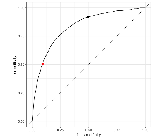
1. Which point represents the quality of our classification rule using a 0.5 probability threshold?

2. The other point corresponds to a different classification rule which uses a different threshold. Is that threshold smaller or bigger than 0.5?

3. Which classification rule do you prefer?

Example 3

The area under an ROC curve (AUC) estimates the probability that our algorithm is more likely to classify y = 1 (rain) as 1 (rain) than to classify y = 0 (no rain) as 1 (rain), hence distinguish between the 2 classes. AUC is helpful for evaluating and comparing the overall quality of classification models. Consider 3 different possible predictors (A, B, C) of rainy and non-rainy days:

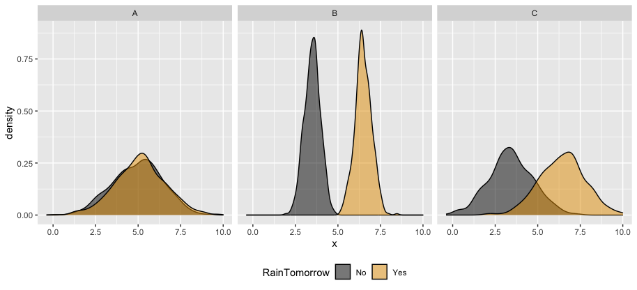
Which predictor is the “strongest” predictor of rain tomorrow?

The ROC curves corresponding to the models RainTomorrow ~ A, RainTomorrow ~ B, RainTomorrow ~ C are shown below.

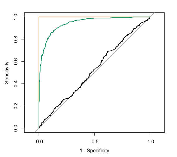
For each ROC curve, indicate the corresponding model and the approximate AUC. Do this in any order you want!

black ROC curve

• RainTomorrow ~ ___
• AUC is roughly ___

green ROC curve

• RainTomorrow ~ ___
• AUC is roughly ___.

orange ROC curve

• RainTomorrow ~ ___
• AUC is exactly ___.

Small Group Activity

Today’s in-class exercises will be due as Homework 5.

Please find the exercises and template there.

I recommend working on Exercises 1, 5, and 6 in class. Exercise 1 is necessary to the other exercises, and Exercises 5 and 6 involve new content: ROC curves, AUC, and LASSO for classification!

After Class

Concept Quiz 1

• Revise Quiz 1 Part 1 (due Friday at 5pm)
• For any X, write a more correct answer and why the original was not quite right.
• My goal: Your understanding / learning
• You may talk with any current Stat 253 student, preceptor, or instructor.

Group Assignment

• Due tonight.
• Most important: your justification of your final model; show your understanding of concepts in your justification.
• If you are encountering errors, let me know.
  • Computational intensity is a valid justification for or against models, but if you are getting errors, then you are missing something.

Upcoming due dates

• Today: Group Assignment 1
  • Step 1: Submit brief report.
  • Step 2: Submit test MAE.
• Friday: HW 5
• Please install 2 packages before Thursday’s class: rpart and rpart.plot