Examine a residual plot, ie. a scatterplot of the residuals vs predictions for each case. Points should appear random and balanced above and below 0 across the entire span of predictions.
Let’s clear up a few things:
We don’t need the exactly same number of residuals above and below 0
Consider balance in terms of weight (each residual doesn’t have equal weight)
Mean of Residuals = 0 (always “balanced” overall)
All residuals are “random” if the data is based on a random sample
You can’t break apart the words above:
Key phrase “appear random above and below 0”
Key phrase “appear balanced above and below 0”
Key phrase “across the entire span of predictions”
Is it Wrong? - Residuals
Updated Text from Course Website:
Points should appear randomly scattered with no clear pattern. If you see any patterns in the residuals that suggest you are systematically over or underpredicting for different prediction values, this indicates that the assumption about the relationship with predictors could be wrong.
Announcements
MSCS Events
Thursday at 11:15am - MSCS Coffee Break
Smail Gallery
Thursday, March 7, 4:45pm, OLRI 250: Joseph Johnson, “Advertising and Sex Cells: Analogies between the Development of Size Difference in Sex Cells and the Development of Name Brand and Generics”
Monday, March 25, 4:45pm, JBD: MSCS & Society Lecture
Announcements
Next Group Formation
Fill out form with preference for next group for Group Assignment 2
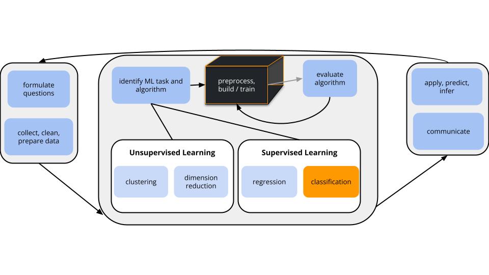
Where are we?
CONTEXT
world = supervised learning
We want to model some output variable \(y\) using a set of potential predictors (\(x_1, x_2, ..., x_p\)).
task = CLASSIFICATION \(y\) is categorical
algorithm = NONparametric
GOAL
The parametric logistic regression model assumes:
\[\text{log(odds that y is 1)} = \beta_0 + \beta_1 x_1 + \beta_2 x_2 + ... + \beta_k x_k\]
NONparametric algorithms will be necessary when this model is too rigid to capture more complicated relationships.
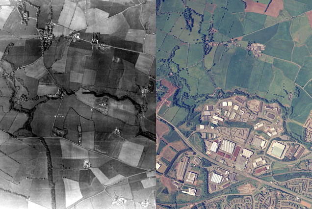
Motivation
Aerial photography studies of land cover is important to land conservation, land management, and understanding environmental impact of land use.
IMPORTANT: Other aerial photography studies focused on people and movement can be used for surveillance, raising major ethical questions.
# Check it outhead(land_3)
      type  NDVI Mean_G Bright_100 SD_NIR
1    tree   0.31 240.18     161.92  11.50
2    tree   0.39 184.15     117.76  11.30
3 asphalt  -0.13  68.07      86.41   6.12
4   grass   0.19 213.71     175.82  11.10
5    tree   0.35 201.84     125.71  14.31
6    tree   0.23 200.16     124.30  12.97
Thus we have the following variables:
type = observed type of land cover, hand-labelled by a human (asphalt, grass, or tree)
factors computed from the image
Though the data includes measurements of size and shape, we’ll focus on texture and “spectral” measurements, i.e. how the land interacts with sun radiation.
NDVI = vegetation index
Mean_G = the green-ness of the image
Bright_100 = the brightness of the image
SD_NIR = a texture measurement (calculated by the standard deviation of “near infrared”)
Limits of Logistic Regression
Why can’t we use logistic regression to model land type (y) by the possible predictors NDVI, Mean_G, Bright_100, SD_NIR (x)?
Parametric v. Nonparametric Classification
There are parametric classifications algorithms that can model y outcomes with more than 2 categories. But they’re complicated and not very common.
We’ll consider two nonparametric algorithms today: K Nearest Neighbors & classification trees.
Nonparametric Classification
Pro: flexibility
Avoid assumptions about the “shape” of this relationship.
Cons
lack of insights:
no coefficients, limited info about relationships
ignoring information about relationships:
When the shape of a relationship is “known”, we should use that shape.
more computationally intense
Small Group Activity - KNN
Let’s develop some intuition about classification with KNN
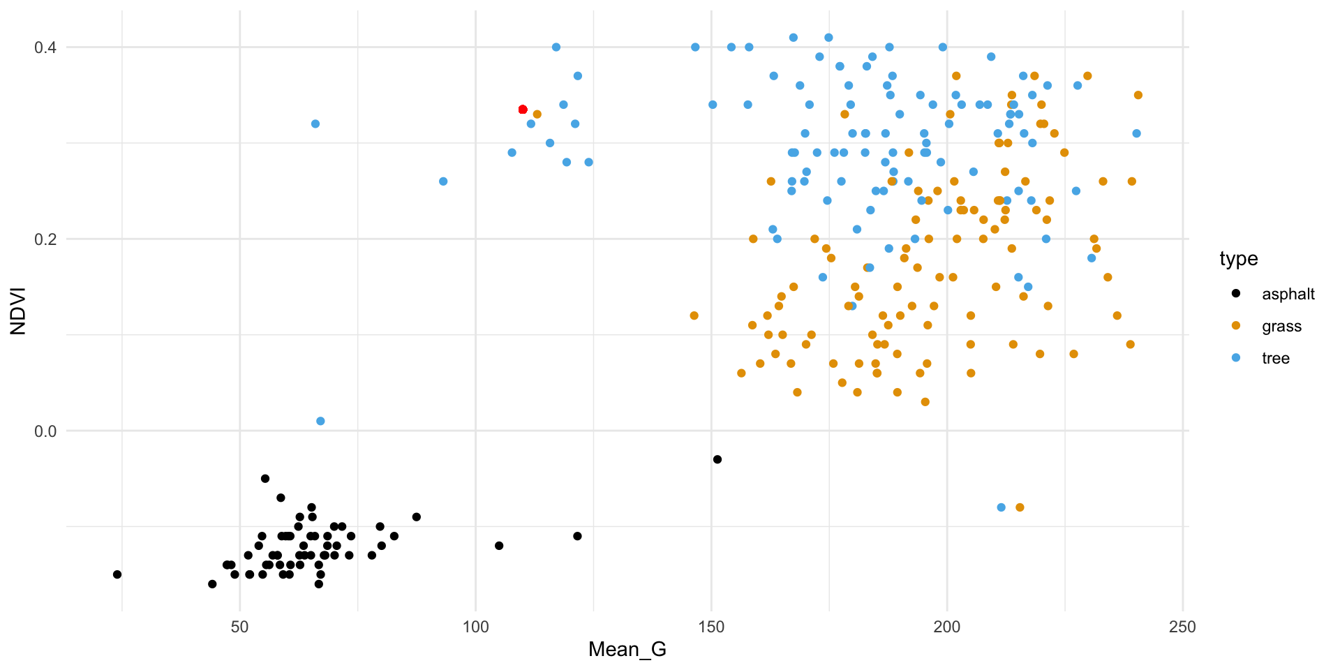
Exercise 1
We’ll start by classifying land type using vegetation index (NDVI) and green-ness (Mean_G).
First, plot and describe this relationship.
Exercise 2
The red dot below represents a new image with NDVI = 0.335 and Mean_G = 110:
How would you classify this image (asphalt, grass, or tree) using…
the 1 nearest neighbor
the 3 nearest neighbors
all 277 neighbors in the sample
Exercise 3
Just as with KNN in the regression setting, it will be important to standardize quantitative x predictors before using them in the algorithm.
Why?
Exercise 4
Let’s confirm our results of grass (a), tree (b), and grass (c) doing this “by hand”…
Try writing R code to find the closest neighbors (without tidymodels).