More KNN & Trees
Where are we?
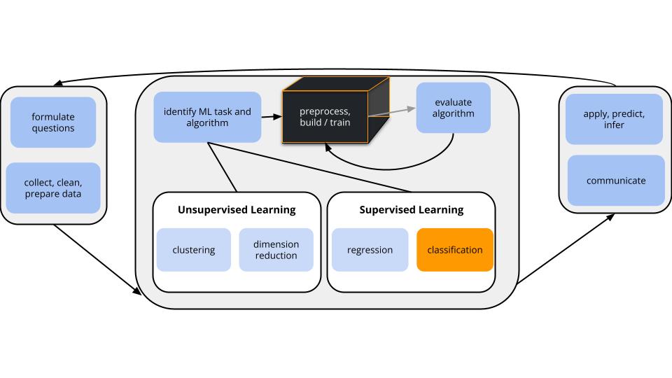
CONTEXT
world = supervised learning
We want to model some output variable \(y\) using a set of potential predictors (\(x_1, x_2, ..., x_p\)).task = CLASSIFICATION
\(y\) is categoricalalgorithm = NONparametric
GOAL
Build and evaluate nonparametric classification models of some categorical outcome y.
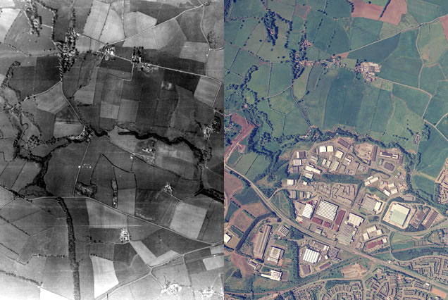
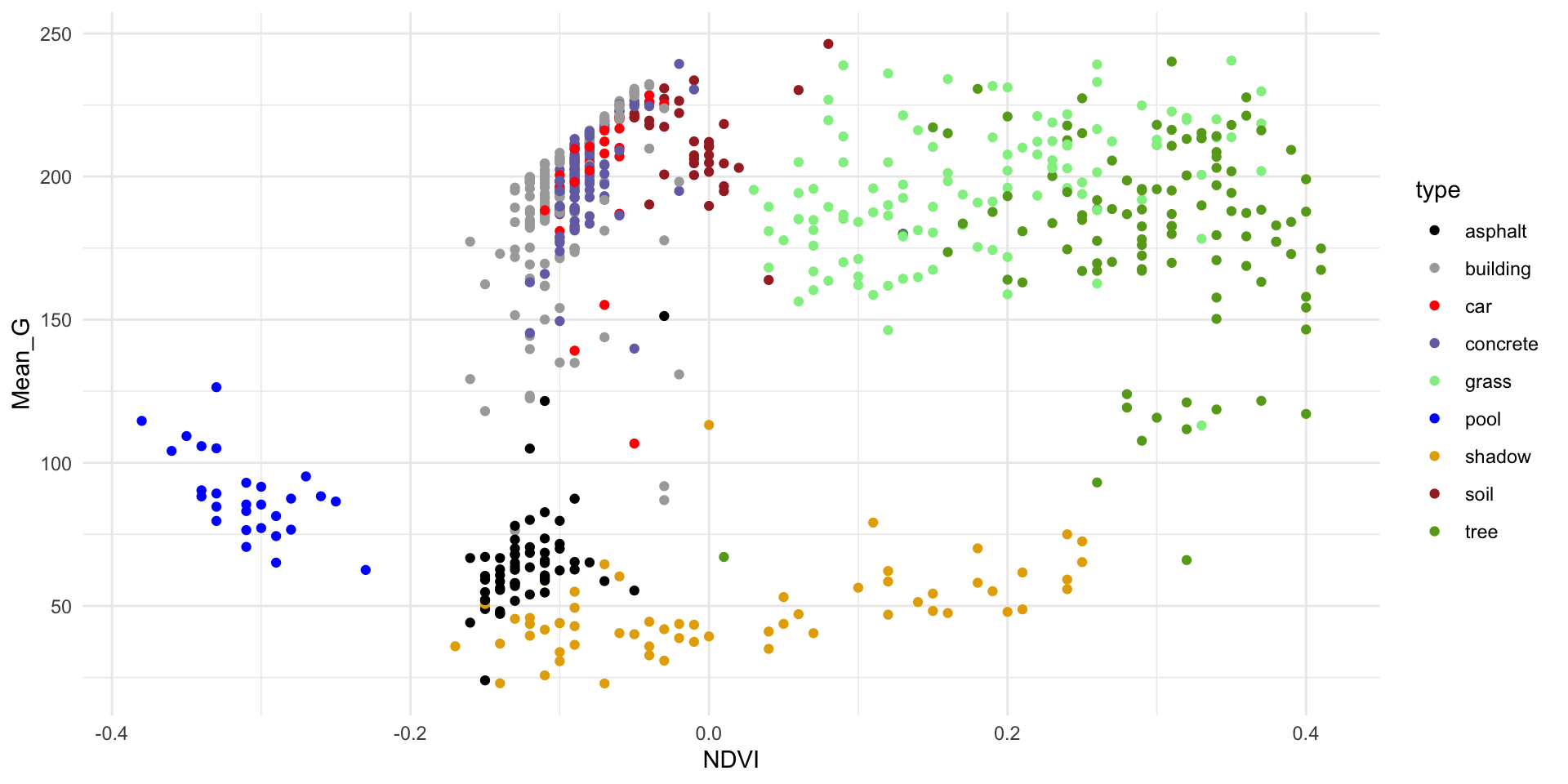
Data Motivation
Aerial photography studies of land cover is important to land conservation, land management, and understanding environmental impact of land use.
IMPORTANT: Other aerial photography studies focused on people and movement can be used for surveillance, raising major ethical questions.
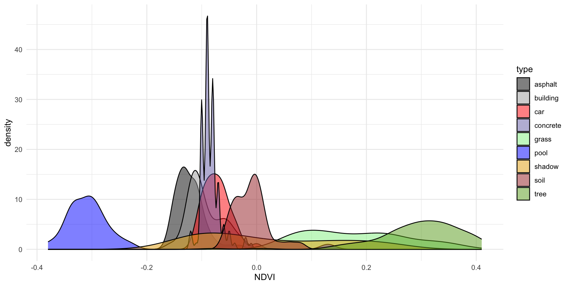
# There are 9 land types!
# Let's consider all of them (not just asphalt, grass, trees)
land %>%
  count(type)
type n
1 asphalt 59
2 building 122
3 car 36
4 concrete 116
5 grass 112
6 pool 29
7 shadow 61
8 soil 34
9 tree 106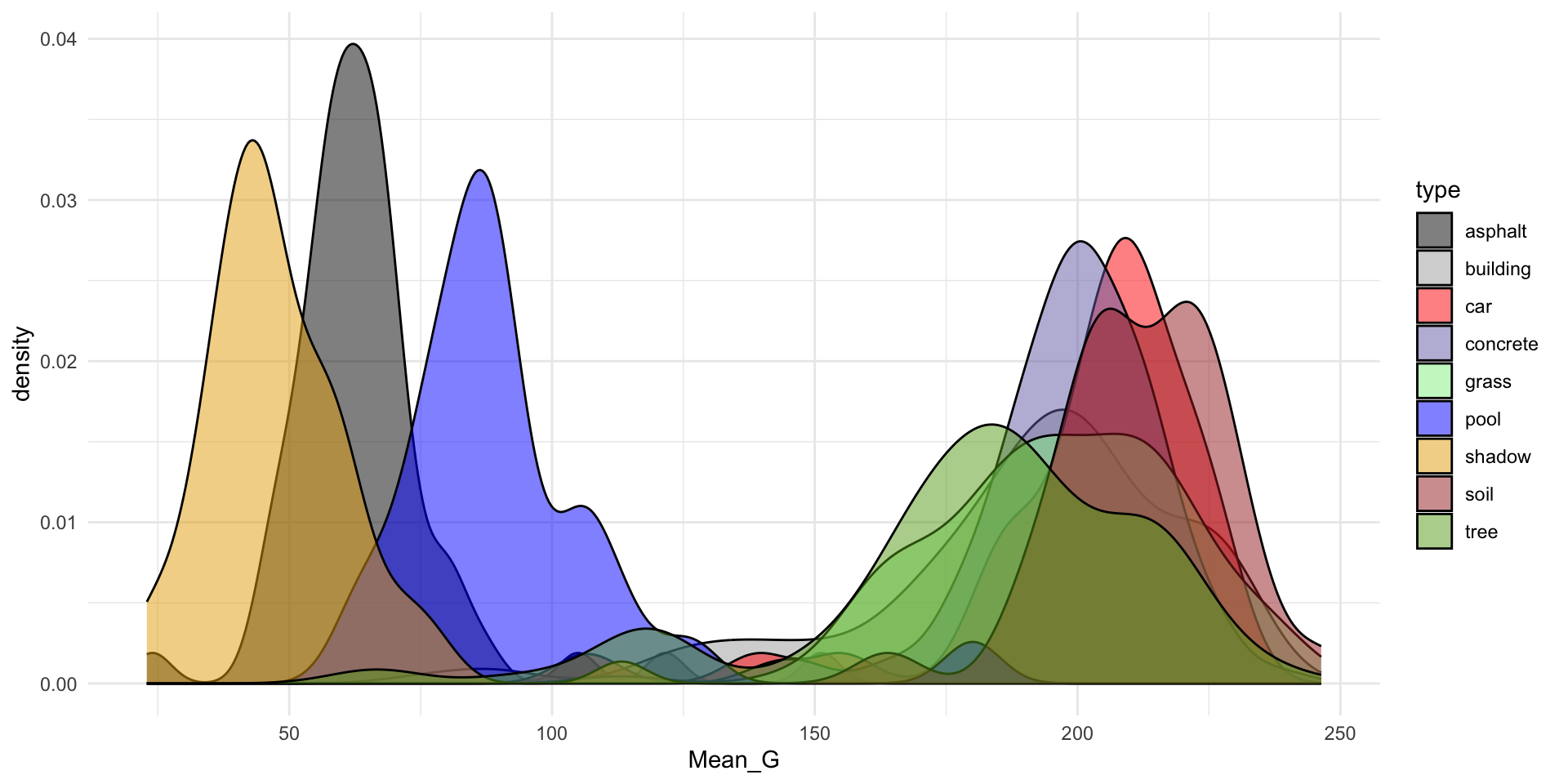
EXAMPLE 1: KNN
Check out the classification regions for two KNN models of land type by Mean_G and NDVI: using K = 1 neighbor and using K = 16 neighbors.
Though the KNN models were built using standardized predictors, the predictors are plotted on their original scales here.
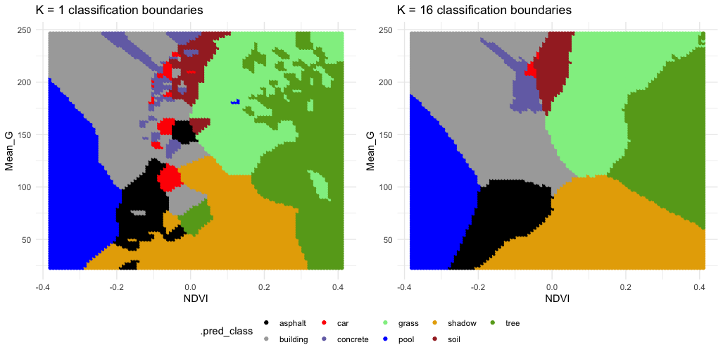
Follow-up:
- What do KNN regression and classification have in common?
- How are they different?
- What questions do you have about…the impact of K, the algorithm, or anything else KNN related?
EXAMPLE 2: Pruned tree
Next, consider a PRUNED classification tree of land type by Mean_G and NDVI that was pruned as follows:
- set maximum depth to 30
- set minimum number of data points per node to 2
- tune the cost complexity parameter.
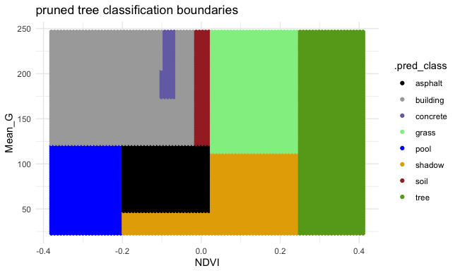
Follow-up:
- What category is missing from the leaf nodes?
- Why did this happen?
- What questions do you have about…the algorithm, pruning, or anything else tree related?
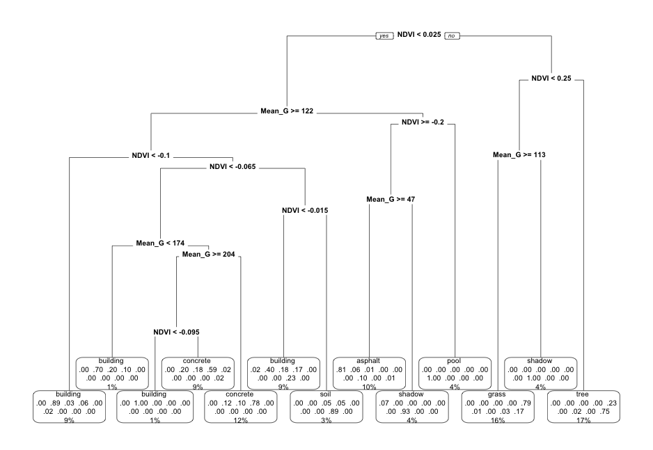
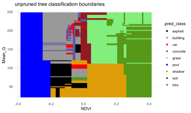
EXAMPLE 3: Unpruned tree
Finally, consider a (mostly) UNPRUNED classification tree of land type by Mean_G and NDVI that was built using the following tuning parameters:
- set maximum depth to 30
- set minimum number of data points per node to 2
- set cost complexity parameter to 0.
Check out the classification regions defined by this tree:
And the tree itself.
This tree was plotted using a function that draws the length of each branch split to be proportional to its improvement to the classification accuracy. The labels are left off to just focus on structure:
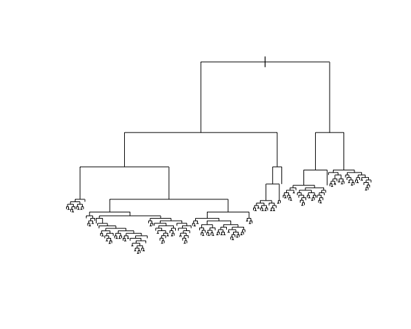
- What happens to the length of the split branches the further down the tree we get? What does this mean?
- What are your thoughts about this tree?
- What questions do you have about the impact of the tuning parameters, or anything else tree related?
After Class
Upcoming due dates
- Tonight: HW 5 (Grace Period ends)
- 3/28: HW 6