Try to sit with at least 1 person you don’t know well
Introduce yourself
Announcements
MSCS Events
Thursday at 11:15am - MSCS Coffee Break
April 18: MSCS Seminar (Prof. Laura Lyman)
Context
GOALS
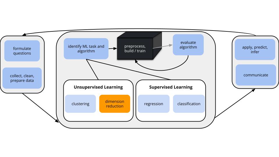
In unsupervised learning we don’t have any y outcome variable, we’re just exploring the structure of our data.
This can be divided into 2 types of tasks:
clustering
GOAL: examine structure & similarities among the individual observations (rows) of our dataset
METHODS: hierarchical and K-means clustering
dimension reduction
GOAL: examine & simplify structure among the features (columns) of our dataset
METHODS: principal components analysis (and many others, including singular value decomposition (SVD), Uniform Manifold Approximation and Projection (UMAP))
Dimension Reduction
Especially when we have a lot of features, dimension reduction helps:
identify patterns among the features
conserve computational resources
feature engineering: create salient features to use in regression & classification (will discuss next class)
Principal Component Analysis
PCA Details
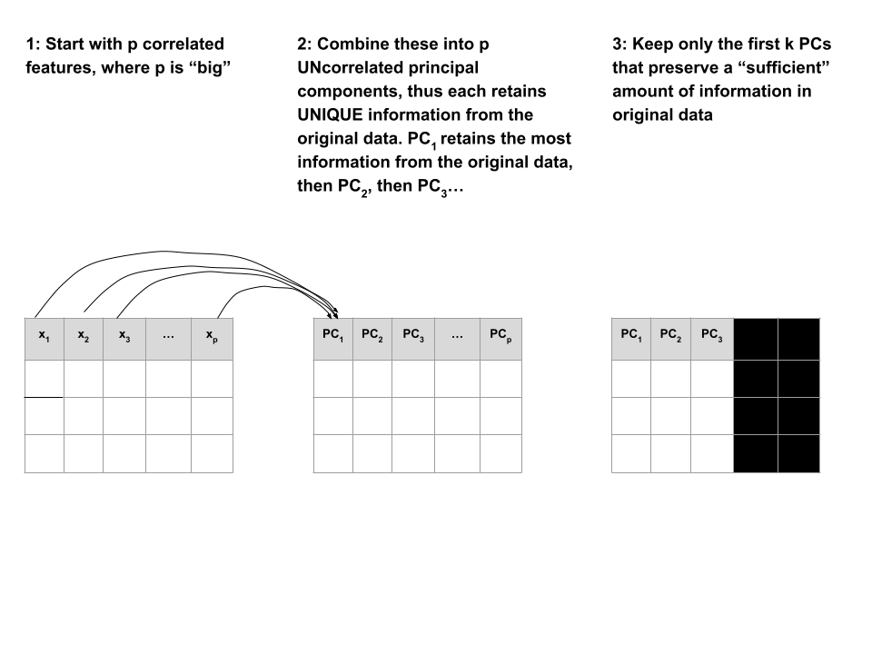
Suppose we start with high dimensional data with p correlated features: \(x_1\), \(x_2\), …, \(x_p\).
We want to turn these into a smaller set of k < p features or principal components\(PC_1\), \(PC_2\), …., \(PC_k\) that:
are uncorrelated (i.e. each contain unique information)
preserve the majority of information or variability in the original data
Step 1
Define the p principal components as linear combinations of the original x features.
These combinations are specified by loadings or coefficients notated as \(a_{ij}\)’s:
The first PC\(PC_1\) is the direction of maximal variability – it retains the greatest variability or information in the original data.
The subsequent PCs are defined to have maximal variation among the directions orthogonal to / perpendicular to / uncorrelated with the previously constructed PCs.
Step 2
Keep only the subset of PCs which retain “enough” of the variability / information in the original dataset.
Data Details
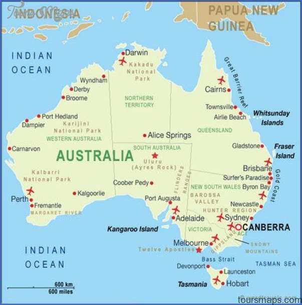
Recall the Australian weather data from Homework 2
# Import the data and load some packageslibrary(tidyverse)library(rattle)data(weatherAUS)# Note that this has missing valuescolSums(is.na(weatherAUS))
We could simply eliminate days with any missing values, but this would kick out a lot of useful info.
Instead, we’ll use KNN to impute the missing values using the VIM package.
# If your VIM package works, use this chunk to process the datalibrary(VIM)# It would be better to impute before filtering & selecting# BUT it's very computationally expensive in this caseweather_temp <- weatherAUS %>%filter(Date =="2008-12-01") %>% dplyr::select(-Date, -RainTomorrow, -Temp3pm, -WindGustDir, -WindDir9am, -WindDir3pm) %>% VIM::kNN(imp_var =FALSE)# Now convert Location to the row name (not a feature)weather_temp <- weather_temp %>%column_to_rownames("Location") # Create a new data frame that processes logical and factor features into dummy variablesweather_data <-data.frame(model.matrix(~ . -1, data = weather_temp))rownames(weather_data) <-rownames(weather_temp)
Identify a research goal that could be addressed using one of our clustering algorithms.
Identify a research goal that could be addressed using our PCA dimension reduction algorithm
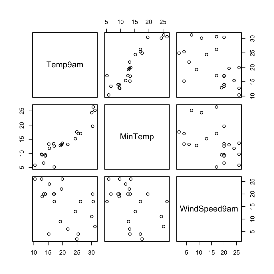
Example 2
Let’s start with just 3 correlated features:
\(x_1\) (Temp9am), \(x_2\) (MinTemp), and \(x_3\) (WindSpeed9am)
The goal of PCA will be to combine these correlated features into a smaller set of uncorrelated principal components (PCs) without losing a significant amount of information.
The first PC will be defined to retain the greatest variability, hence information in the original features. What do you expect the first PC to be like?
How many PCs do you think we’ll need to keep without losing too much of the original information?
Example 3
Perform a PCA on the small_example data:
# This code is nice and short!# scale = TRUE, center = TRUE first standardizes the featurespca_small <-prcomp(small_example, scale =TRUE, center =TRUE)
This creates 3 PCs which are each different combinations of the (standardized) original features:
# Original (standardized) featuresscale(small_example) %>%head()
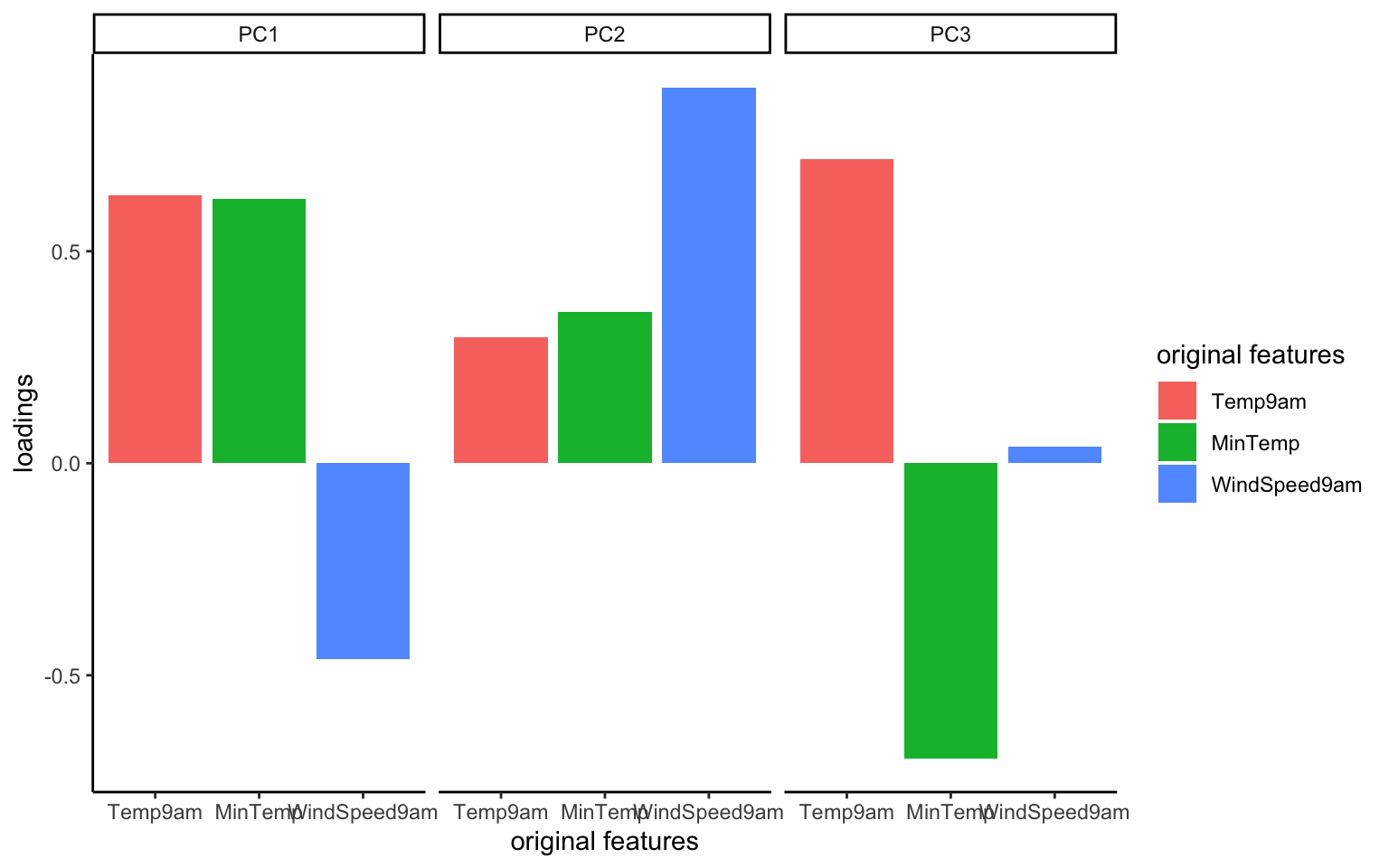
Plots can help us interpret the above numerical loadings, hence the important components of each PC.
Which features contribute the most, either positively or negatively, to the first PC?
What about the second PC?
Example 5
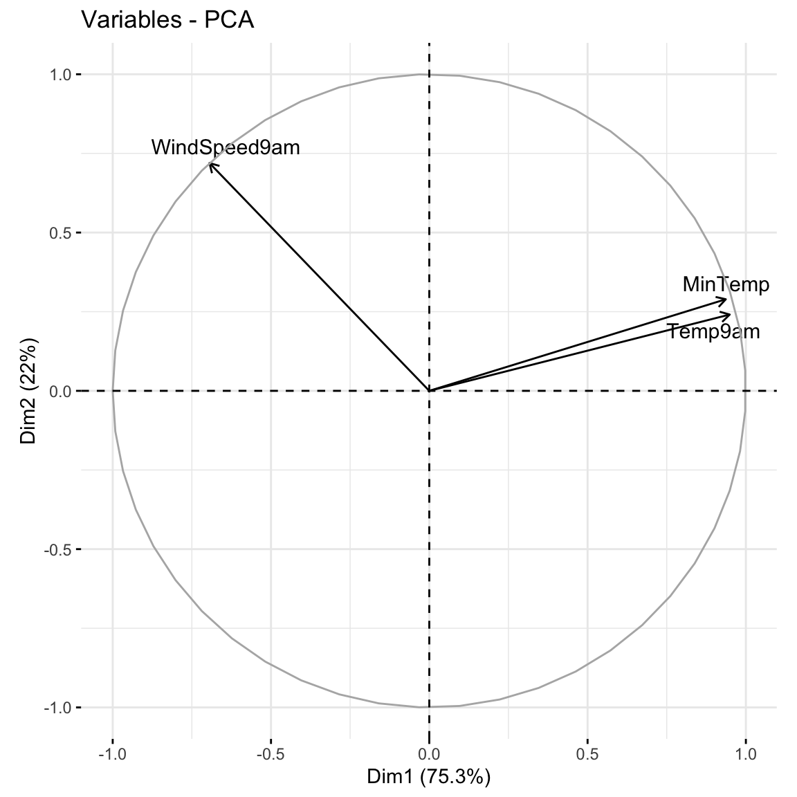
When we have a lot of features x, the above plots get messy. A loadings plot or correlation circle is another way to visualize PC1 and PC2 (the most important PCs):
each arrow represents a feature x
the x-coordinate of an arrow reflects the correlation between x and PC1
the y-coordinate of an arrow reflects the correlation between x and PC2
arrow length reflects how much the feature contributes to the first 2 PCs
It is powerful in that it can provide a 2-dimensional visualization of high dimensional data (just 3 dimensions in our small example here)!
Positively correlated features point in similar directions. The opposite is true for negatively correlated features. What do you learn here?
Which features are most highly correlated with, hence contribute the most to, the first PC (x-axis)? (Is this consistent with what we observed in the earlier plots?)
What about the second PC?
Example 6
Now that we better understand the structures of the PCs, let’s examine the relative amount of information they each capture from the original set of features:
# Load package for tidy tablelibrary(tidymodels)# Measure information captured by each PC# Calculate variance from standard deviationpca_small %>%tidy(matrix ="eigenvalues") %>%mutate(var = std.dev^2)
var = amount of variability, hence information, in the original features captured by each PC
percent = % of original information captured by each PC
cumulative = cumulative % of original information captured by the PCs
What % of the original information is captured by PC1? Confirm using both the var and percent columns.
What % of the original information is captured by PC2?
In total, 100% of the original information is captured by PC1, PC2, and PC3. What % of the original info would we retain if we only kept PC1 and PC2, i.e. if we reduced the PC dimensions by 1? Confirm using both the percent and cumulative columns.
Example 7
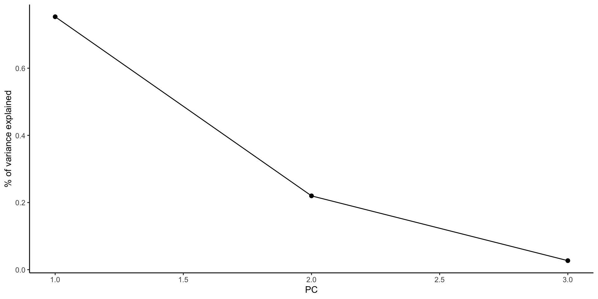
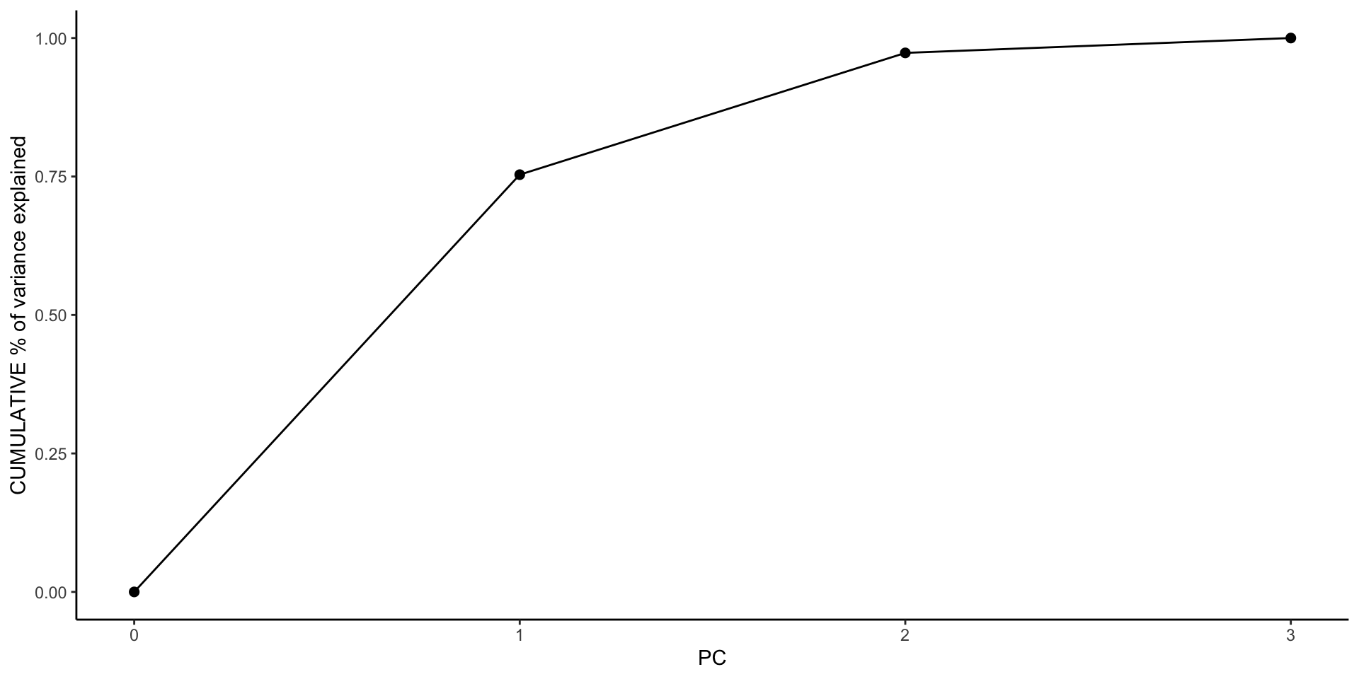
Especially when we start with lots of features, graphical summaries of the above tidy summary can help understand the variation captured by the PCs:
Based on these summaries, how many and which of the 3 PCs does it make sense to keep?
Thus by how much can we reduce the dimensions of our dataset?
Example 8
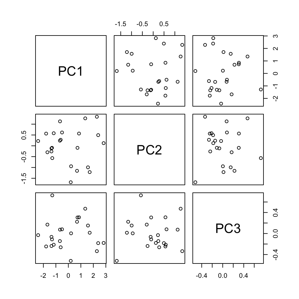
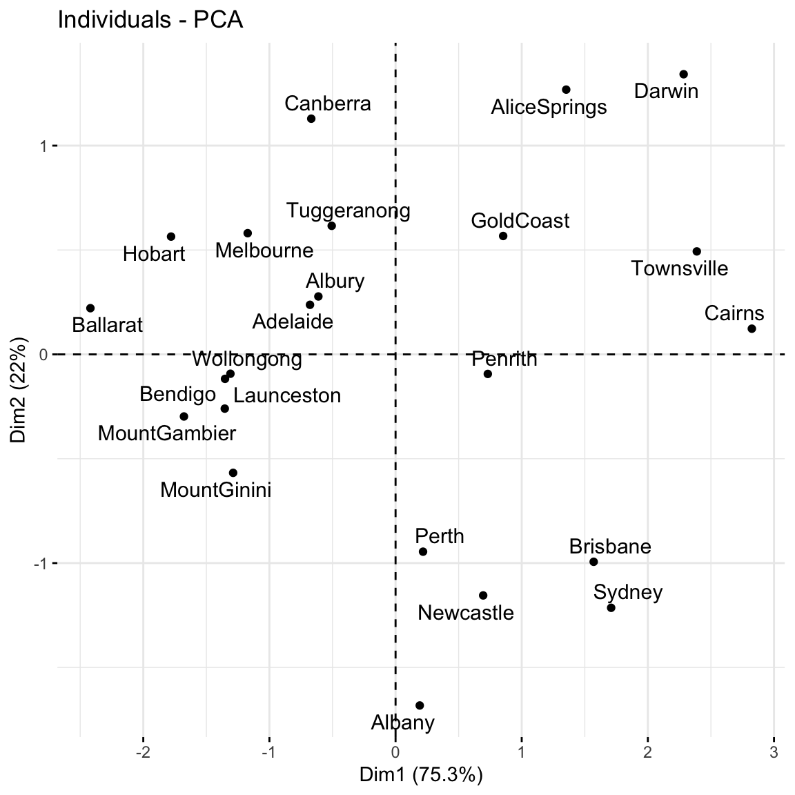
Finally, now that we better understand the “meaning” of our 3 new PCs, let’s explore their outcomes for each city (row) in the dataset.
A score plot maps out the scores of the first, and most important, 2 PCs for each city. PC1 is on the x-axis and PC2 on the y-axis.
Does there appear to be any geographical explanation of which cities are similar with respect to their PC1 and PC2 scores?
Small Group Work
For the rest of the class, work together Example 9 and 10 (solutions on site) and then on Ex 7-8 on HW7 (Rmd on Moodle).