6.5 Bernoulli/Binomial Model
There are situations in which your response of interest only has two possible outcomes: success or failure, heart disease or no heart disease, o-ring failure or no o-ring failure, etc. In the past, we used logistic regression to create a model to predict a binary response variable based on explanatory variables. For a moment, let’s just consider the response itself as a random process.
If a random process satisfies the following three conditions, then we can use the Bernoulli Model to understand its long-run behavior:
- Two possible outcomes (success or failure)
- Independent “trials” (the outcome for one unit does not depend on the outcome for any other unit)
- P(success) = \(p\) is constant (the relative frequency of success in the population that we are drawing from is constant)
If a random variable \(X\) follows a Bernoulli model, \(X\) denotes the number of successes (0 or 1) in the single trial that is conducted. The probability mass function is \(P(X = 1) = p\) and \(P(X = 0) = 1-p\). In the long run, the expected number of successes will be \(p\), the variance will be \(p(1-p)\), and the standard deviation will be \(\sqrt{p(1-p)}\). If you have looked through the [Appendix A], you can show this mathematically using definitions.
Let’s think back to the disease testing example. Say we have a very large population where 1 in every 1000 has a particular disease (\(p = 1/1000\)). We could model the disease outcome from randomly drawing an individual from the population using a Bernoulli Model where \(P(X = 1) = 0.001\). If we just randomly drew 1 person, we’d expect 0.001 of a person to have the disease and the spread in outcomes is \(\sqrt{0.001*0.999} = 0.031\). These values don’t make a lot of sense because we often sample more than one person.
Imagine we had a sample of \(n\) individuals from the population. Then we are considering \(n\) independent Bernoulli “trials”. If we let the random variable \(X\) be the count of the number of successes in a sample of size \(n\), then we can use the Binomial Model. In this case we say that “\(X\) follows a binomial distribution”.
The probability mass function for the Binomial Model is
\[p(x) = P(X = x) = \frac{n!}{x!(n-x)!}p^x(1-p)^{n-x}\]
where \(x\) is the number of successes in \(n\) trials. In the long run, the expected number of successes will be \(np\), the variance will be \(np(1-p)\), and the standard deviation will be \(\sqrt{np(1-p)}\). In the long run, the expected relative frequency of successes in \(n\) trials will be \(p\), the variance will be \(\frac{p(1-p)}{n}\) and the standard deviation will be \(\sqrt{\frac{p(1-p)}{n}}\). If you are working through the [Appendix A], you can show these mathematically using known properties.
If we randomly draw 5000 people, we’d expect \(0.001*5000 = 5\) people to have the disease and the spread in the count is \(\sqrt{5000*0.001*0.999} = 2.23\). Let’s adjust this to relative frequencies. We’d expect 0.1% (5/5000 = 0.001) of the people to have the disease and a measure of the variability in relative frequency is \(\sqrt{0.001*0.999/5000} = 0.0004\).
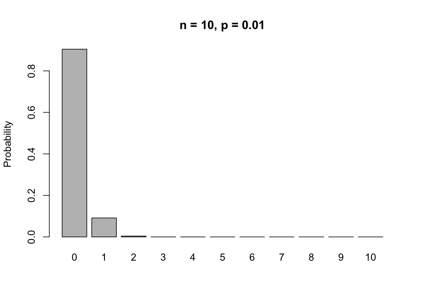
Let’s look at the probability mass function for the Binomial Model for \(n = 10, p = 0.01\).
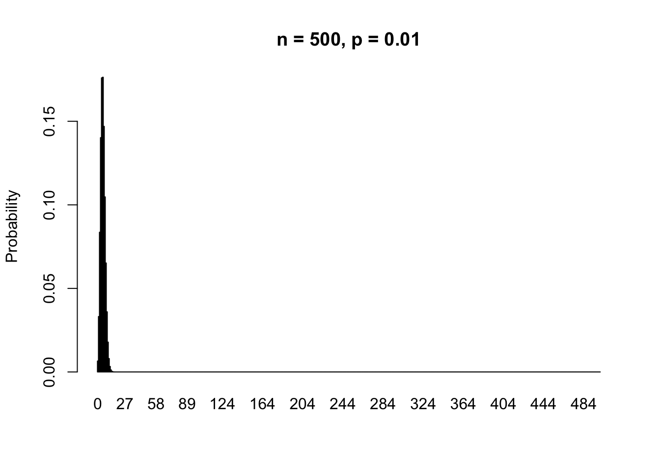
If we increase the sample size to \(n = 500\), then the probability mass function looks like this.
Let’s zoom in on the left hand side of this plot.
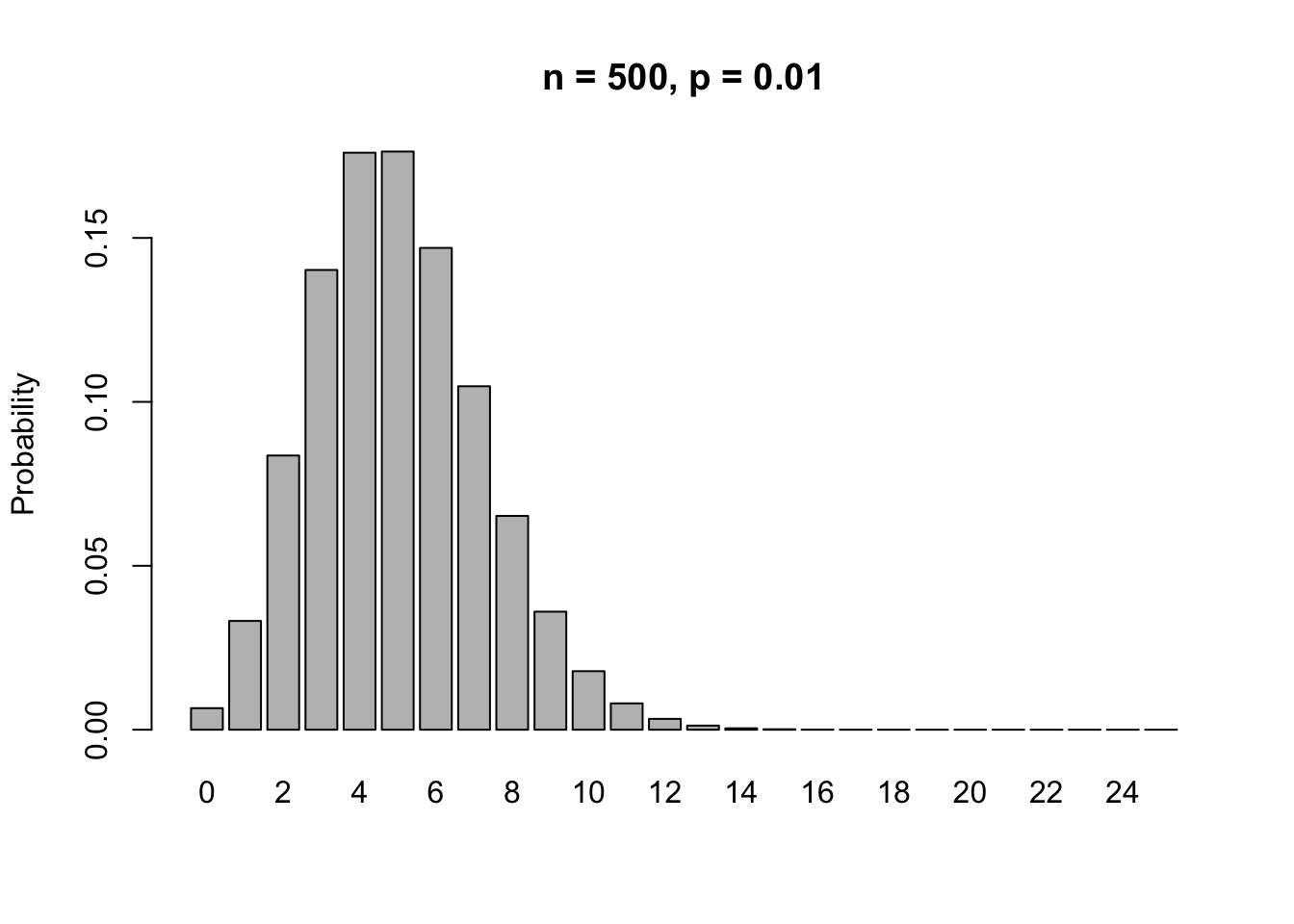
What does this look like? A Normal Model!!!