5.4 IRL: Bootstrapping

In real life (IRL), we don’t have a full target population from which we can repeatedly draw samples. We only have one sample that was already drawn from the larger target population.

To get a sense of the sampling variability, we could try to mimic this process of sampling from the full target population using our best stand-in for the population: our sample. We will call the sample our “fake population” for the moment. This process of resampling our sample is called bootstrapping.

We bootstrap our sample in order to 1) estimate the variability of the statistic and 2) get a range of plausible values for the true population parameter.

There are four steps to bootstrapping. They are very similar to simulating the sampling process from a population.

1. Generate

To generate different random samples of the same size (100 flights) from our “fake population”, we have to draw sample of 100 flights WITH REPLACEMENT, meaning that we have to put a flight back into the pool after drawing them out.

What would happen if we drew WITHOUT REPLACEMENT?

2. Calculate

In our simulation above, we calculated the median and mean arrival delay. In theory, we could calculate any numerical summary of data (e.g. the mean, median, SD, 25th percentile, etc.)

boot_data <- mosaic::do(1000)*( 
    flights_samp1 %>% # Start with the SAMPLE (not the FULL POPULATION)
      sample_frac(replace = TRUE) %>% # Generate by resampling with replacement
      with(lm(arr_delay ~ day_hour)) # Fit linear model
)

Notice the similarities and differences in the R code for boot_data, in which we are sampling from the sample, and sim_data, in which we are sampling from the population, above.

3. Summarize

Let’s summarize these 1000 model estimates generated from resampling (with replacement) from our sample (our “fake population”).

# Summarize
boot_data %>% 
    summarize(
        mean_Intercept = mean(Intercept),
        mean_dayhourmorning = mean(day_hourmorning),
        sd_Intercept = sd(Intercept),
        sd_dayhourmorning = sd(day_hourmorning))

##   mean_Intercept mean_dayhourmorning sd_Intercept sd_dayhourmorning
## 1       14.58742           -20.49495     7.218149           8.44133

Note how the mean’s are very close to the original estimates from the sample, below.

flights_samp1 %>%
    with(lm(arr_delay ~ day_hour)) %>%
    tidy()

## # A tibble: 2 x 5
##   term            estimate std.error statistic p.value
##   <chr>              <dbl>     <dbl>     <dbl>   <dbl>
## 1 (Intercept)         14.4      6.38      2.26  0.0258
## 2 day_hourmorning    -20.4     10.6      -1.92  0.0578

This is not a coincidence. Since we are resampling from our original sample, we’d expect the bootstrap estimates to bounce around the original sample estimates, similar to how the simulated sampling distributions had means close the the population values

Let’s compare this to the summaries from the simulation of randomly sampling from the population.

sim_data %>% 
    summarize(
        mean_Intercept = mean(Intercept),
        mean_dayhourmorning = mean(day_hourmorning),
        sd_Intercept = sd(Intercept),
        sd_dayhourmorning = sd(day_hourmorning))

##   mean_Intercept mean_dayhourmorning sd_Intercept sd_dayhourmorning
## 1       13.45053           -14.54158     7.233256           8.87308

The means won’t be exactly the same because the center of the bootstrap distribution is the original sample and the center of the sampling distribution is the population values.

But, the standard deviations should be of roughly similar magnitude because they are in fact trying to estimate the same thing, the sampling variability.

4. Visualize

Let’s visualize these 1000 models generated from resampling (with replacement) from our sample (our “fake population”).

# Visualize Intercepts
boot_data %>% 
    ggplot(aes(x = Intercept)) +
    geom_histogram(bins = 15) +
    labs(title = "Bootstrap sampling distribution of Intercepts\nfrom samples of 100 flights") +
    theme_minimal()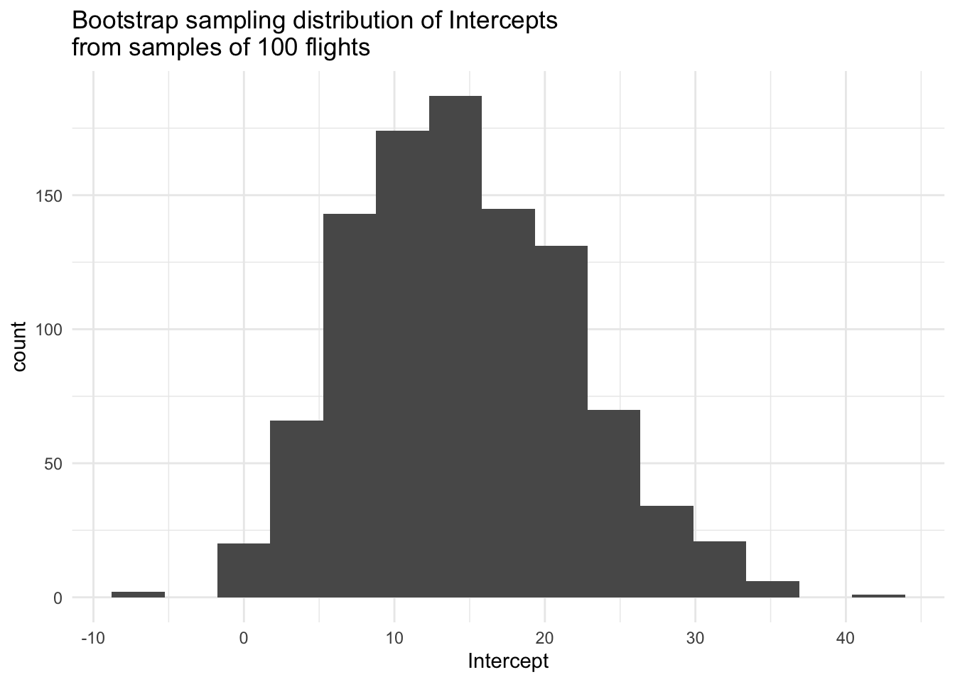

# Visualize Slopes
boot_data %>% 
    ggplot(aes(x = day_hourmorning)) +
    geom_histogram(bins = 15) +
    labs(title = "Bootstrap sampling distribution of Slopes\nfrom samples of 100 flights") +
    theme_minimal()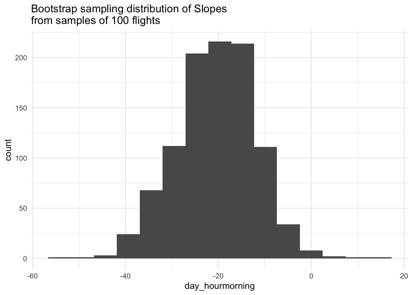

Let’s compare these to the visuals from the simulation from the population.

# Visualize Intercepts
sim_data %>% 
    ggplot(aes(x = Intercept)) +
    geom_histogram(bins = 15) +
    labs(title = "Sampling distribution of Intercepts\nfrom samples of 100 flights") +
    theme_minimal()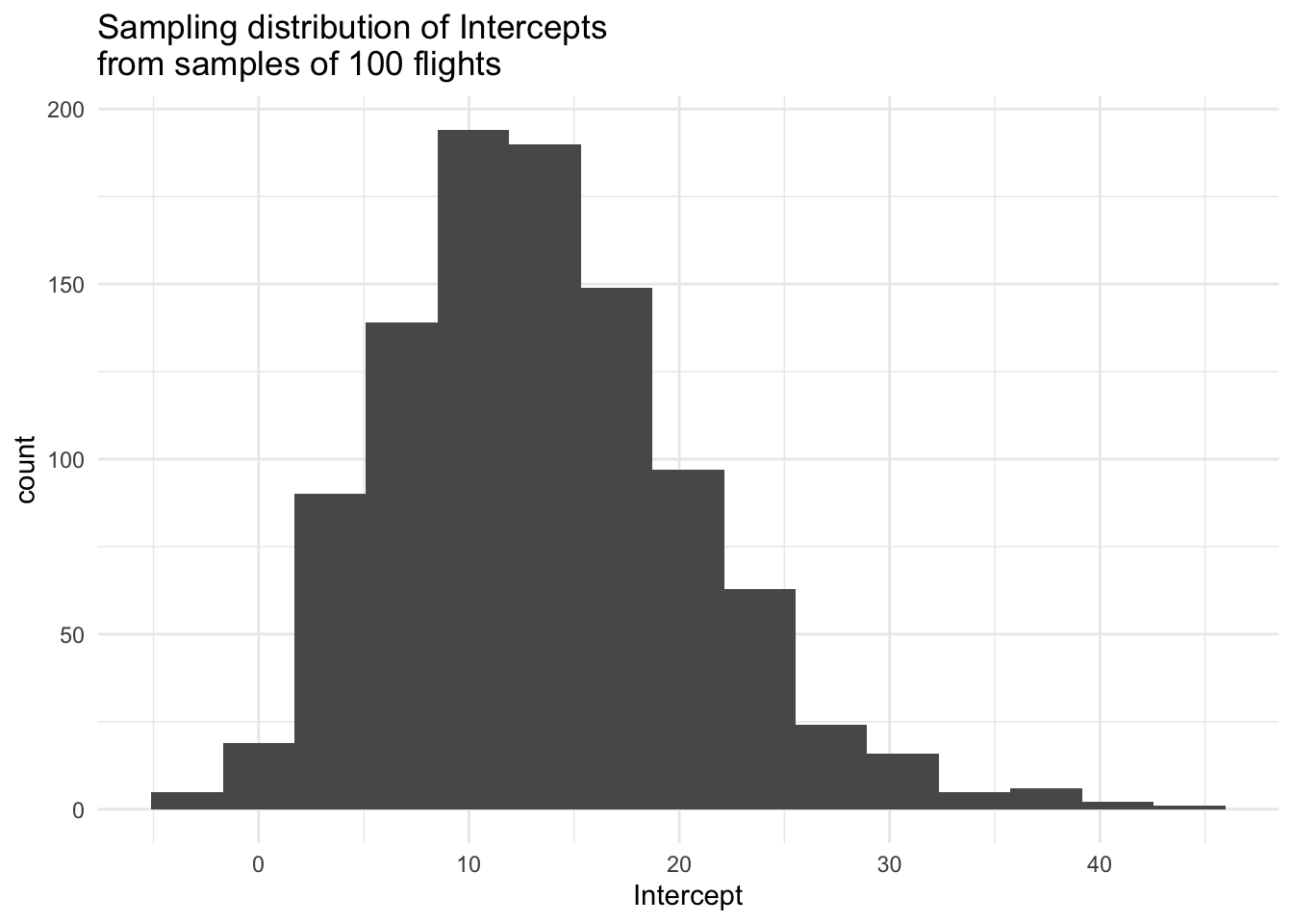

# Visualize Slopes
sim_data %>% 
    ggplot(aes(x = day_hourmorning)) +
    geom_histogram(bins = 15) +
    labs(title = "Sampling distribution of Slopes\nfrom samples of 100 flights") +
    theme_minimal()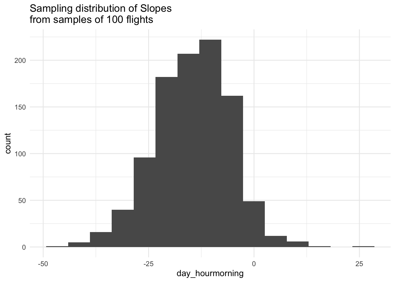

The process of resampling from our sample, called bootstrapping, is becoming the one of main computational tools for estimating sampling variability in the field of Statistics.

How well does bootstrapping do in mimicking the simulations from the population? What could we change to improve bootstrap’s ability to mimic the simulations?

This is a really important concept in Statistics! We’ll come back to the ideas of sampling variability and bootstrapping throughout the rest of the course.

Based on the bootstrap sampling distribution, what would you guess the difference in mean arrival delay between morning and afternoon is in the population of flights?

Based on the bootstrap sampling distribution, if you had to give an interval of plausible values for the population difference, what range would you give? Why? Is a difference of 0 a plausible value?