8.5 Random Variation

How has randomness come up in the course so far?

• Random sampling (sampling variation)
• Random assignment of treatment
• Random variation in general (due to biology, measurement error, etc.)

We want to be able to harness the randomness by understanding the random behavior in the long run.

• If we were to repeatedly take samples from the population, how would the estimates (mean, odds ratio, slope etc.) differ?
• If we were to repeat the random assignment many times, how would the estimated effects differ?

Now, based on the theory we know, we could show a few things about means, \(\bar{X} = \frac{1}{n}\sum_{i=1}^n X_i\).

Say we have a sequence of independent and identically distributed (iid) random variables, \(X_1,...,X_n\), (I don’t know what their probability model is but the expected value and variance is the same, \(E(X_i) = \mu\) and \(Var(X_i) = \sigma^2\))

Then we’d expect the mean to be approximately \(\mu\),

\[E(\frac{1}{n}\sum_{i=1}^n X_i) = \mu\] and the mean would vary, but that variation would decrease with increased sample size \(n\),

\[Var(\frac{1}{n}\sum_{i=1}^n X_i) = \frac{\sigma^2}{n}\]

But, what is the shape of the distribution (probability model) of the mean?

Let’s randomly generate data from a probability model with a skewed pdf.

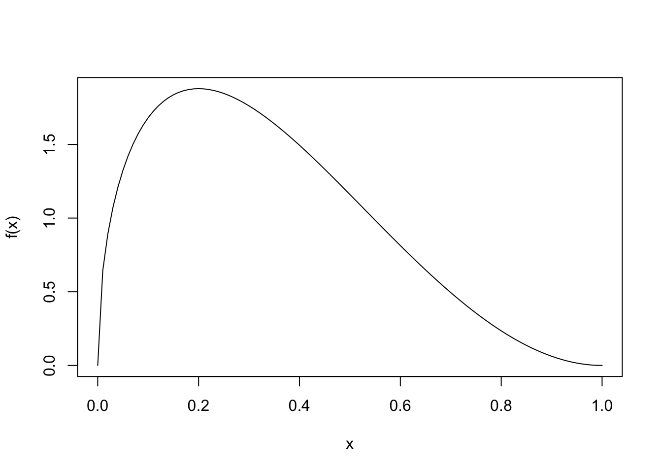
Let \(\bar{y}\) be the mean of those \(n\) random values. If we repeat the process multiple times, we get a sense of the sampling distribution for \(\bar{y}\), the mean of a sample of \(n\) random values from the population distribution above.

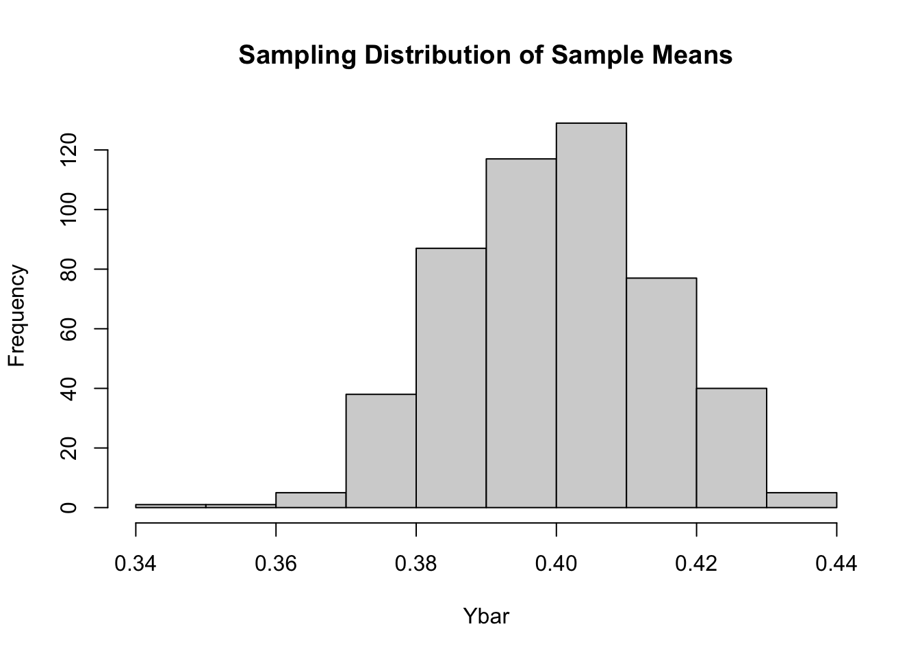
The Central Limit Theorem (CLT) tells us that as the sample size get larger and larger, the shape of the sampling distribution for the sample mean get closer and closer to Normal. That is why it makes sense we’ve seen unimodal, symmetric distributions pop up when we simulate bootstrapping and random assignments. However, the CLT only applies when we are talking about sample means or proportions.

Let our sample mean be \(Y_n = \frac{1}{n}\sum_{i=1}^n X_i\) based on a sample size of \(n\).

• Let’s subtract the expected value, \(E(Y) = \mu\), and scale by \(\sqrt{n}\), such that we have a new random variable, \[C_n = \sqrt{n}\left(Y_n - \mu\right) \]

• The Central Limit Theorem tells us that for any \(c \in \mathbb{R}\), \[\lim_{n\rightarrow\infty}P(C_n \leq c) = P(Y \leq c)\] where \(Y\) is a Normal RV with \(E(Y) = 0\) and \(Var(Y) = \sigma^2\).

## 
## Attaching package: 'dplyr'

## The following objects are masked from 'package:stats':
## 
##     filter, lag

## The following objects are masked from 'package:base':
## 
##     intersect, setdiff, setequal, union

## Loading required package: xml2

## Loading required package: lattice

## Loading required package: ggformula

## Loading required package: ggstance

## 
## Attaching package: 'ggstance'

## The following objects are masked from 'package:ggplot2':
## 
##     geom_errorbarh, GeomErrorbarh

## 
## New to ggformula?  Try the tutorials: 
## 	learnr::run_tutorial("introduction", package = "ggformula")
## 	learnr::run_tutorial("refining", package = "ggformula")

## Loading required package: Matrix

## Registered S3 method overwritten by 'mosaic':
##   method                           from   
##   fortify.SpatialPolygonsDataFrame ggplot2

## 
## The 'mosaic' package masks several functions from core packages in order to add 
## additional features.  The original behavior of these functions should not be affected by this.
## 
## Note: If you use the Matrix package, be sure to load it BEFORE loading mosaic.
## 
## Have you tried the ggformula package for your plots?

## 
## Attaching package: 'mosaic'

## The following object is masked from 'package:Matrix':
## 
##     mean

## The following object is masked from 'package:ggplot2':
## 
##     stat

## The following objects are masked from 'package:dplyr':
## 
##     count, do, tally

## The following objects are masked from 'package:infer':
## 
##     prop_test, t_test

## The following objects are masked from 'package:stats':
## 
##     binom.test, cor, cor.test, cov, fivenum, IQR, median, prop.test,
##     quantile, sd, t.test, var

## The following objects are masked from 'package:base':
## 
##     max, mean, min, prod, range, sample, sum