6.8 Z-scores and the Student’s “t” distribution
Let’s stop for a short story time. Back in the early 1900’s, William S. Gosset was working as a quality control chemist and mathematician for Guinness Brewery in Ireland.
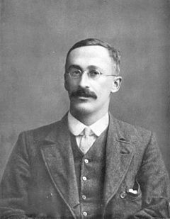 Source: Wikipedia
His research goal was to determine how to get the best yielding barley and hops through agricultural experimentation, but the main issue that he had was that he had very small sample sizes (only a handful of farms)!
He was used the Normal distribution because the work underlying the Central Limit Theorem had already been worked out, but he noticing that there were discrepancies in his work.
6.8.1 Gosset’s Work
To further investigate the issues that he was noticing, Gosset performed a simulation using data on the height and left middle finger measurements of 3000 criminals (we don’t know how he got access to this data…). His simulations went as follows:
- Split the data (3000 criminals) into samples of size 4 (\(n=4\))
- Estimate the mean and standard deviation of the height within each of the 750 samples
- Look at the distribution of the z score heights, using the mean of the 3000 as the true population mean, \(\mu\), but using \(s\) in the denominator from each sample instead of the population variation, \(\sigma\), of the 3000:
\[ z = \frac{\bar{x} - \mu}{s/\sqrt{4}}\]
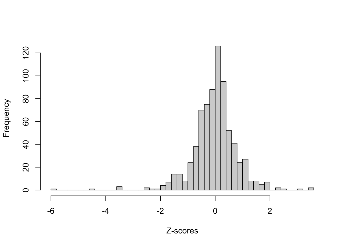
- Does this distribution of z-scores look Normal? We can try to see more clearly by making a Q-Q plot, shown below.
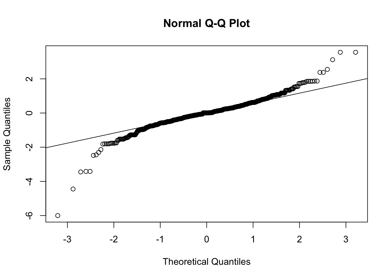
If the z-scores follow a normal distribution, the points in the Q-Q plot should fall on a straight line. However, we see some deviation at the left and right of the plots. This indicates that the tails of our z-score distribution are thicker (more populous) than expected if they were actually normally-distributed.
Why? With small samples, the sample standard deviation, \(s\), is smaller so we tend to get larger z-scores than we’d expect if they were normally-distributed.
6.8.2 Beer Helps the Field of Statistics
For the sake of making better beer, William Gosset worked out the sampling distribution of a standardized sample mean (with the sample standard deviation, \(s\), plugged into the denominator),
\[t = \frac{\bar{x} - \mu}{s/\sqrt{n}}\]
if the histogram of the population is unimodal and roughly symmetric (approximately Normal). This was crucial when sample sizes are small. He had to publish under the pseudonym Student (trade secrets, etc.). Thus, the sampling distribution model that he discovered became known as Student’s model. Later R.A. Fisher (another famous statistician) recoined it as the Student’s T model.
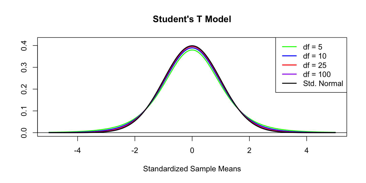
6.8.3 Student’s T Model
- The center is always 0.
- The spread is determined by a parameter called degrees of freedom (for standardized means, \(df = n - 1\)).
- As \(n\rightarrow\infty\), this model looks more like the Normal model.
Since the Student T distribution is approximately Normal when sample sizes are large, we will typically use the Normal model. However, if sample sizes are small (\(n<30\) or so), the Normal model is not appropriate. So, in those rare cases, we’ll need to refer to Student’s T.