The data this week comes from the arthistory data package.
This dataset contains data that was used for Holland Stam’s thesis work, titled Quantifying art historical narratives. The data was collected to assess the demographic representation of artists through editions of Janson’s History of Art and Gardner’s Art Through the Ages, two of the most popular art history textbooks used in the American education system. In this package specifically, both artist-level and work-level data was collected along with variables regarding the artists’ demographics and numeric metrics for describing how much space they or their work took up in each edition of each textbook.
This package contains three datasets: - worksjanson: Contains individual work-level data by edition of Gardner’s art history textbook from 1963 until 2011. For each work, there is information about the size of the work and text as displayed in the textbook as well as details about the work’s medium and year created. Demographic data about the artist is also included. - worksgardner: Contains individual work-level data by edition of Gardner’s art history textbook from 1926 until 2020. For each work, there is information about the size of the work as displayed in the textbook as well as the size of the accompanying descriptive text. Demographic data about the artist is also included. - artists: Contains various information about artists by edition of Gardner or Janson’s art history textbook from 1926 until 2020. Data includes demographic information, space occupied in the textbook, as well as presence in the MoMA and Whitney museums.
Rows: 3162 Columns: 14
── Column specification ────────────────────────────────────────────────────────
Delimiter: ","
chr (8): artist_name, artist_nationality, artist_nationality_other, artist_g...
dbl (6): edition_number, year, space_ratio_per_page_total, artist_unique_id,...
ℹ Use `spec()` to retrieve the full column specification for this data.
ℹ Specify the column types or set `show_col_types = FALSE` to quiet this message.
head(artists)
# A tibble: 6 × 14
  artist_name   edition_number  year artist_nationality artist_nationality_other
  <chr>                  <dbl> <dbl> <chr>              <chr>
1 Aaron Douglas              9  1991 American           American
2 Aaron Douglas             10  1996 American           American
3 Aaron Douglas             11  2001 American           American
4 Aaron Douglas             12  2005 American           American
5 Aaron Douglas             13  2009 American           American
6 Aaron Douglas             14  2013 American           American
# ℹ 9 more variables: artist_gender <chr>, artist_race <chr>,
#   artist_ethnicity <chr>, book <chr>, space_ratio_per_page_total <dbl>,
#   artist_unique_id <dbl>, moma_count_to_year <dbl>,
#   whitney_count_to_year <dbl>, artist_race_nwi <chr>
`summarise()` has grouped output by 'year_cat', 'artist_unique_id',
'artist_name', 'artist_nationality', 'artist_nationality_other',
'artist_gender', 'artist_race'. You can override using the `.groups` argument.
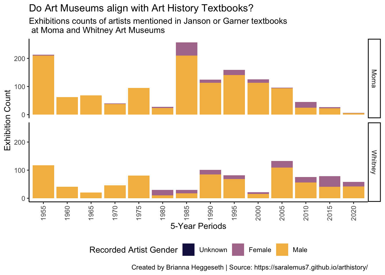
foo %>%group_by(year_cat,artist_gender) %>%summarize(Moma =sum(diff_moma),Whitney =sum(diff_whitney)) %>%pivot_longer(cols=c('Moma','Whitney'), names_to ='museum' ,values_to ='exh_count') %>%mutate(artist_gender =factor(fct_recode(factor(artist_gender),'Unknown'='N/A'))) %>%ggplot(aes(x = year_cat, y = exh_count, fill =fct_reorder(artist_gender,exh_count))) +geom_col() +labs(y ='Exhibition Count', x ='5-Year Periods',fill ='Recorded Artist Gender',title='Do Art Museums align with Art History Textbooks?',subtitle='Exhibitions counts of artists mentioned in Janson or Garner textbooks\n at Moma and Whitney Art Museums', caption ='Created by Brianna Heggeseth | Source: https://saralemus7.github.io/arthistory/' ) +facet_grid(museum~.) +scale_fill_manual( values=met.brewer("Renoir", n=3,type='discrete')) +theme_classic() +theme(axis.text.x =element_text(angle =90, vjust =0.5, hjust=1)) +theme(legend.position="bottom")
`summarise()` has grouped output by 'year_cat'. You can override using the
`.groups` argument.
Warning: There were 4 warnings in `mutate()`.
The first warning was:
ℹ In argument: `artist_gender = factor(fct_recode(factor(artist_gender),
  Unknown = "N/A"))`.
ℹ In group 2: `year_cat = 1960`.
Caused by warning:
! Unknown levels in `f`: N/A
ℹ Run `dplyr::last_dplyr_warnings()` to see the 3 remaining warnings.
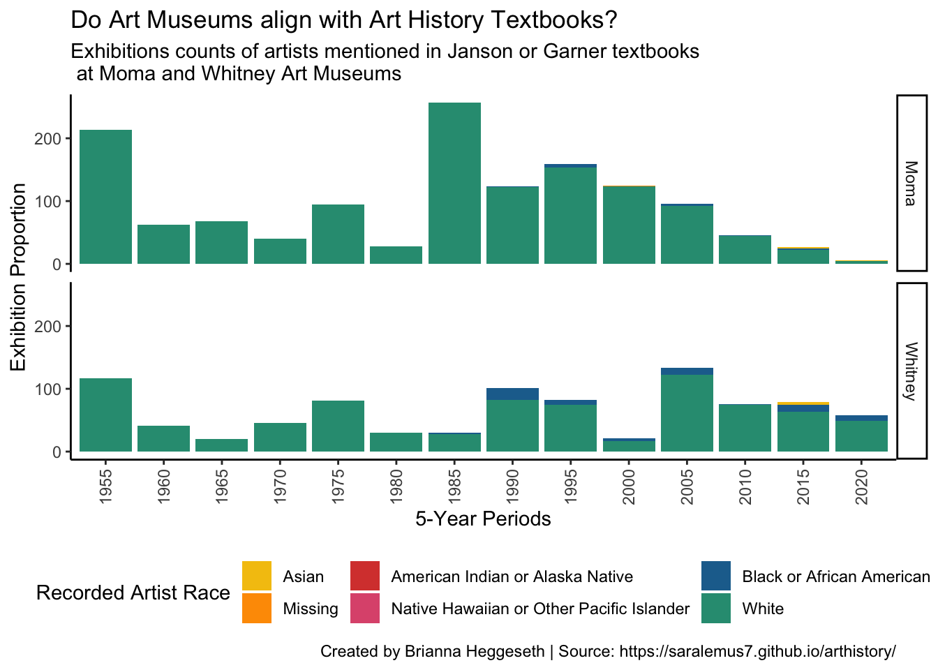
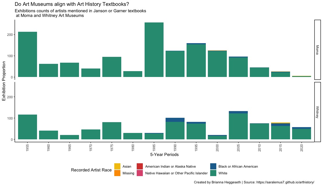
foo %>%group_by(year_cat,artist_race) %>%summarize(Moma =sum(diff_moma),Whitney =sum(diff_whitney)) %>%pivot_longer(cols=c('Moma','Whitney'), names_to ='museum' ,values_to ='exh_count') %>%mutate(artist_race =factor(fct_recode(factor(artist_race),'Missing'='N/A'))) %>%ggplot(aes(x = year_cat, y = exh_count, fill =fct_reorder(artist_race,exh_count))) +geom_col() +labs(y ='Exhibition Proportion', x ='5-Year Periods', fill ='Recorded Artist Race',title='Do Art Museums align with Art History Textbooks?',subtitle='Exhibitions counts of artists mentioned in Janson or Garner textbooks\n at Moma and Whitney Art Museums', caption ='Created by Brianna Heggeseth | Source: https://saralemus7.github.io/arthistory/' ) +facet_grid(museum~.) +scale_fill_manual( values=met.brewer("Signac", n=6,type='discrete')) +theme_classic() +theme(axis.text.x =element_text(angle =90, vjust =0.5, hjust=1)) +theme(legend.position="bottom")
`summarise()` has grouped output by 'year_cat'. You can override using the
`.groups` argument.
Warning: There were 4 warnings in `mutate()`.
The first warning was:
ℹ In argument: `artist_race = factor(fct_recode(factor(artist_race), Missing =
  "N/A"))`.
ℹ In group 2: `year_cat = 1960`.
Caused by warning:
! Unknown levels in `f`: N/A
ℹ Run `dplyr::last_dplyr_warnings()` to see the 3 remaining warnings.