Topic 9 Joining Two Data Frames

Learning Goals

Understand the concept of keys and variables that uniquely identify rows or cases
Understand the different types of joins, different ways of combining two data frames together
Develop comfort in using mutating joins: left_join, inner_join and full_join in the dplyr package
Develop comfort in using filtering joins: semi_join, anti_join in the dplyr package

You can download a template .Rmd of this activity here. Put it in a folder Day_09 in COMP_STAT_112.

Joins

A join is a verb that means to combine two data tables.

These tables are often called the left and the right tables.

There are several kinds of join.

All involve establishing a correspondence — a match — between each case in the left table and zero or more cases in the right table.
The various joins differ in how they handle multiple matches or missing matches.

Establishing a match between cases

A match between a case in the left data table and a case in the right data table is made based on the values in keys, variables that uniquely define observations in a data table.

As an example, we’ll examine the following two tables on grades and courses. The Grades file has one case for each class of each student, and includes variables describing the ID of the student (sid), the ID of the session (section/class), and the grade received. The Courses file has variables for the ID of the session (section/class), the department (coded), the level, the semester, the enrollment, and the ID of the instructor (iid). We show a few random rows of each table below.

Table 9.1: Student grades.
sid	sessionID	grade
S31842	session2207	B+
S32436	session3172	S
S31671	session3435	A-
S31929	session3512	NC

Table 9.2: Information about each course section.
sessionID	dept	level	sem	enroll	iid
session2780	O	300	SP2003	21	inst298
session3520	k	300	FA2004	16	inst463
session1965	d	100	FA2001	25	inst414
session3257	o	200	SP2004	16	inst312

Keys

There are two types of keys:

A primary key uniquely identifies an observation in its own table.
A foreign key uniquely identifies an observation in another table.

Example 9.1 What variables are the primary keys for Grades? What variables are the primary keys for Courses?

Solution

sid (student ID) and sessionID (class ID) are the primary keys for Grades as they unique identify each case.

# can check to make sure that there are no combinations of sid and session ID that have more than 1 row
Grades %>%
  count(sid, sessionID) %>%
  filter(n > 1)

## # A tibble: 0 × 3
## # … with 3 variables: sid <chr>, sessionID <chr>, n <int>

sessionID (class ID) and dept are the primary keys for Courses as they unique identify each case. You may have thought that sessionID alone was sufficient; however, if a course is cross-listed, then it may have multiple departments listed.

# check to make sure that there are no combinations 
# of session ID and dept that have more than 1 row
Courses %>%
  count(sessionID, dept) %>%
  filter(n > 1)

## # A tibble: 0 × 3
## # … with 3 variables: sessionID <chr>, dept <chr>, n <int>

Example 9.2 What variables are the foreign keys in Grades for Courses? What variables are the foreign keys in Courses for Grades?

Solution

sessionID (class ID) is part of a foreign key in Grades for Courses. If we group_by and summarize first to deal with cross-listed courses, then sessionID is the foreign key in Grades for Courses.

# can check to make sure that once we combine enrollment between cross-listed courses, each session ID only has 1 row
Courses %>%
  group_by(sessionID, level, sem, iid) %>%
  summarize(total_enroll = sum(enroll)) %>%
  count(sessionID) %>%
  filter(n > 1)

## # A tibble: 0 × 4
## # Groups:   sessionID, level, sem [0]
## # … with 4 variables: sessionID <chr>, level <dbl>, sem <chr>, n <int>

sessionID in Courses is part of a foreign key that uniquely identify rows in Grades.

Matching

In order to establish a match between two data tables,

You specify which variables (or keys) to use.
Each variable is specify as a pair, where one variable from the left table corresponds to one variable from the right table.
Cases must have exactly equal values in the left variable and right variable for a match to be made.

Mutating joins

The first class of joins are mutating joins, which add new variables (columns) to the left data table from matching observations in the right table.⁸

The main difference in the three mutating join options in this class is how they answer the following questions:

What happens when a case in the right table has no matches in the left table?
What happens when a case in the left table has no matches in the right table?

Three mutating join functions:

left_join(): the output has all cases from the left, regardless if there is a match in the right, but discards any cases in the right that do not have a match in the left.
inner_join(): the output has only the cases from the left with a match in the right.
full_join(): the output has all cases from the left and the right. This is less common than the first two join operators.

When there are multiple matches in the right table for a particular case in the left table, all three of these mutating join operators produce a separate case in the new table for each of the matches from the right.

Example 9.3 (Average class size: varying viewpoints) Determine the average class size from the viewpoint of a student and the viewpoint of the Provost / Admissions Office.

Solution

Provost Perspective:

The Provost counts each section as one class and takes the average of all classes. We have to be a little careful and cannot simply do mean(Courses$enroll), because some sessionID appear twice on the course list. Why is that?⁹ We can still do this from the data we have in the Courses table, but we should aggregate by sessionID first:

CourseSizes <- Courses %>%
  group_by(sessionID) %>%
  summarise(total_enroll = sum(enroll))

mean(CourseSizes$total_enroll)

## [1] 21.45251

Student Perspective:

To get the average class size from the student perspective, we can join the enrollment of the section onto each instance of a student section. Here, the left table is Grades, the right table is CourseSizes, we are going to match based on sessionID, and we want to add the variable total_enroll from CoursesSizes.

We’ll use a left_join since we aren’t interested in any sections from the CourseSizes table that do not show up in the Grades table; their enrollments should be 0, and they are not actually seen by any students. Note, e.g., if there were 100 extra sections of zero enrollments on the Courses table, this would change the average from the Provost’s perspective, but not at all from the students’ perspective.

If the by = is omitted from a join, then R will perform a natural join, which matches the two tables by all variables they have in common. In this case, the only variable in common is the sessionID, so we would get the same results by omitting the second argument. In general, this is not reliable unless we check ahead of time which variables the tables have in common. If two variables to match have different names in the two tables, we can write by = c("name1" = "name2").

EnrollmentsWithClassSize <- Grades %>%
  left_join(CourseSizes,
    by = c("sessionID" = "sessionID")
  ) %>%
  select(sid, sessionID, total_enroll)

Table 9.3: Student enrollments with the section size.
sid	sessionID	total_enroll
S31842	session2207	11
S32436	session3172	51
S31671	session3435	15
S31929	session3512	13

AveClassEachStudent <- EnrollmentsWithClassSize %>%
  group_by(sid) %>%
  summarise(ave_enroll = mean(total_enroll, na.rm = TRUE))

Table 9.4: Average class size seen by each individual student.
sid	ave_enroll
S32169	34.25000
S32121	23.33333
S32472	24.53846
S31467	23.82353

The na.rm = TRUE here says that if the class size is not available for a given class, we do not count that class towards the student’s average class size. What is another way to capture the same objective? We could have used an inner_join instead of a left_join when we joined the tables to eliminate any entries from the left table that did not have a match in the right table.

Now we can take the average of the AveClassEachStudent table, counting each student once, to find the average class size from the student perspective:

mean(AveClassEachStudent$ave_enroll)

## [1] 24.41885

We see that the average size from the student perspective (24.4) is greater than the average size from the Provost’s perspective (21.5).

Filtering joins

The second class of joins are filtering joins, which select specific cases from the left table based on whether they match an observation in the right table.

semi_join(): discards any cases in the left table that do not have a match in the right table. If there are multiple matches of right cases to a left case, it keeps just one copy of the left case.
anti_join(): discards any cases in the left table that have a match in the right table.

A particularly common employment of these joins is to use a filtered summary as a comparison to select a subset of the original cases, as follows.

Example 9.4 (semi_join to compare to a filtered summary) Find a subset of the Grades data that only contains data on the four largest sections in the Courses data set.

Solution

LargeSections <- Courses %>%
  group_by(sessionID) %>%
  summarise(total_enroll = sum(enroll)) %>%
  arrange(desc(total_enroll)) %>% head(4)
GradesFromLargeSections <- Grades %>%
  semi_join(LargeSections)

Example 9.5 (semi_join) Use semi_join() to create a table with a subset of the rows of Grades corresponding to all classes taken in department J.

Solution

There are multiple ways to do this. We could do a left join to the Grades table to add on the dept variable, and then filter by department, then select all variables except the additional dept variable we just added. Here is a more direct way with semi_join that does not involve adding and subtracting the extra variable:

JCourses <- Courses %>%
  filter(dept == "J")
JGrades <- Grades %>%
  semi_join(JCourses)

Let’s double check this worked. Here are the first few entries of our new table:

Table 9.5: Student enrollments in Department J.
sid	sessionID	grade
S31185	session1791	A-
S31185	session1792	B+
S31185	session1794	B-
S31185	session1795	C+

The first entry is for session1791. Which department is that course in? What department should it be?

(Courses %>% filter(sessionID == "session1791"))

## # A tibble: 1 × 6
##   sessionID   dept  level sem    enroll iid    
##   <chr>       <chr> <dbl> <chr>   <dbl> <chr>  
## 1 session1791 J       100 FA1993     22 inst223

Great, it worked! But that only checked the first one. What if we want to double check all of the courses included in Table 9.5? We can add on the department and do a group by to count the number from each department in our table.

JGrades %>%
  left_join(Courses) %>%
  count(dept)

## # A tibble: 1 × 2
##   dept      n
##   <chr> <int>
## 1 J       148

More join practice

Exercise 9.1 Use your wrangling skills to answer the following questions.

Hint 1: start by thinking about what tables you might need to join (if any) and identifying the corresponding variables to match. Hint 2: you’ll need an extra table to convert grades to grade point averages. I’ve given you the code below.

How many student enrollments in each department?
What’s the grade-point average (GPA) for each student? The average student GPA? Hint: There are some “S” and “AU” grades that we want to exclude from GPA calculations. What is the correct variant of join to accomplish this?
What fraction of grades are below B+?
What’s the grade-point average for each instructor?
We cannot actually compute the correct grade-point average for each department from the information we have. The reason why is due to cross-listed courses. Students for those courses could be enrolled under either department, and we do not know which department to assign the grade to. There are a number of possible workarounds to get an estimate. One would be to assign all grades in a section to the department of the instructor, which we’d have to infer from the data. Instead, start by creating a table with all cross-listed courses. Then use an anti_join to eliminate all cross-listed courses. Finally, use an inner_join to compute the grade-point average for each department.

(GPAConversion <- tibble(grade = c("A+", "A", "A-", "B+", "B", "B-", "C+", "C", "C-", "D+", "D", "D-", "NC"), gp = c(4.3, 4, 3.7, 3.3, 3, 2.7, 2.3, 2, 1.7, 1.3, 1, 0.7, 0)))

## # A tibble: 13 × 2
##    grade    gp
##    <chr> <dbl>
##  1 A+      4.3
##  2 A       4  
##  3 A-      3.7
##  4 B+      3.3
##  5 B       3  
##  6 B-      2.7
##  7 C+      2.3
##  8 C       2  
##  9 C-      1.7
## 10 D+      1.3
## 11 D       1  
## 12 D-      0.7
## 13 NC      0

Bicycle-Use Patterns

In this activity, you’ll examine some factors that may influence the use of bicycles in a bike-renting program. The data come from Washington, DC and cover the last quarter of 2014.

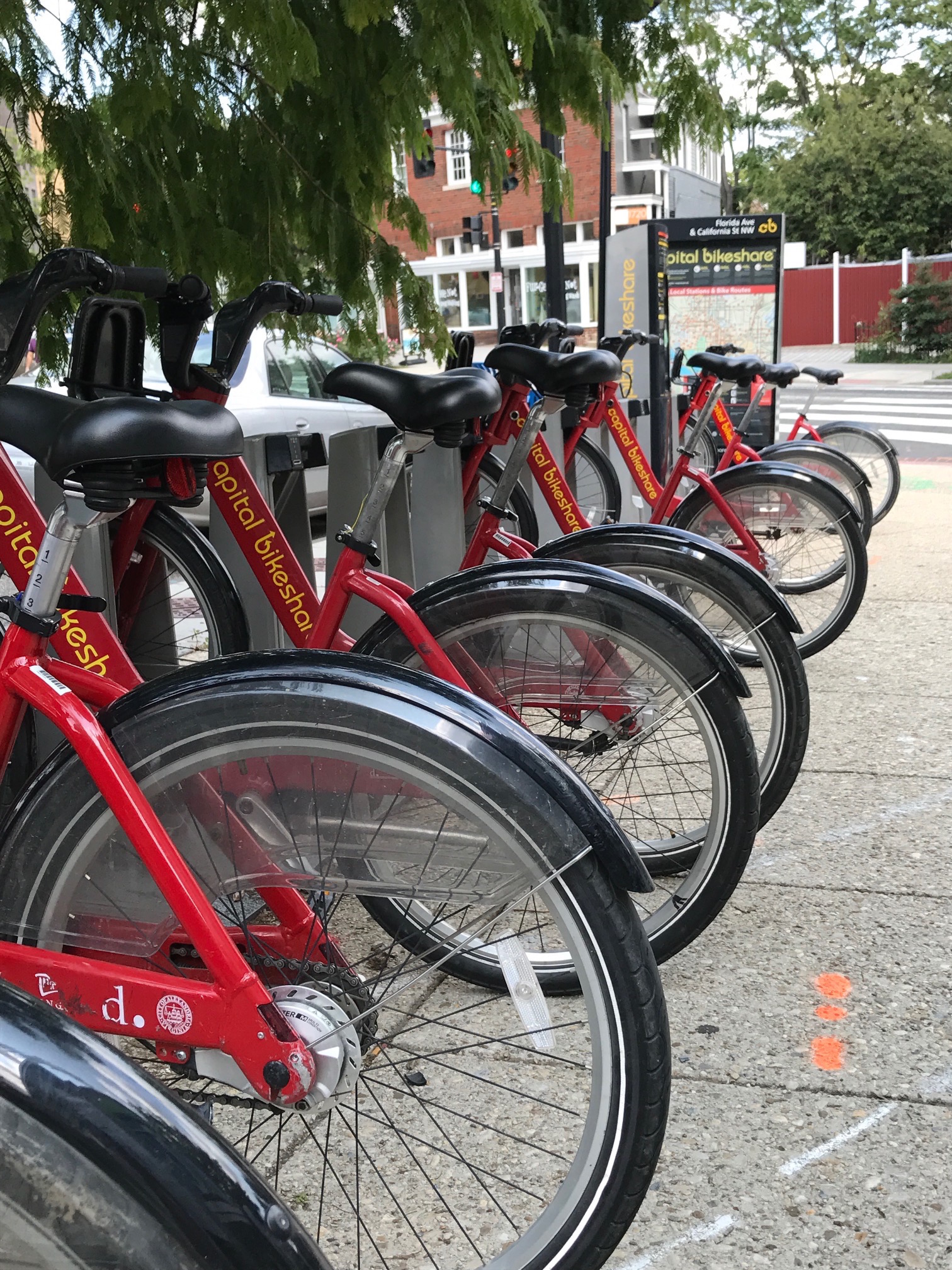
Figure 9.1: A typical Capital Bikeshare station. This one is at Florida and California, next to Pleasant Pops.

Figure 9.2: One of the vans used to redistribute bicycles to different stations.

Two data tables are available:

Trips contains records of individual rentals here
Stations gives the locations of the bike rental stations here

Here is the code to read in the data:¹⁰

data_site <-
  "https://bcheggeseth.github.io/112_fall_2022/data/2014-Q4-Trips-History-Data-Small.rds"
Trips <- readRDS(gzcon(url(data_site)))
Stations <- read_csv("https://bcheggeseth.github.io/112_fall_2022/data/DC-Stations.csv")

The Trips data table is a random subset of 10,000 trips from the full quarterly data. Start with this small data table to develop your analysis commands. When you have this working well, you can access the full data set of more than 600,000 events by removing -Small from the name of the data_site. The full data is available here.

Warm-up: Temporal patterns

It’s natural to expect that bikes are rented more at some times of day, some days of the week, some months of the year than others. The variable sdate gives the time (including the date) that the rental started.

Exercise 9.2 (Warm-up: temporal patterns) Make the following plots and interpret them:

A density plot of the events versus sdate. Use ggplot() and geom_density().
A density plot of the events versus time of day. You can use mutate with lubridate::hour(), and lubridate::minute() to extract the hour of the day and minute within the hour from sdate. Hint: A minute is 1/60 of an hour, so create a field where 3:30 is 3.5 and 3:45 is 3.75.
A histogram of the events versus day of the week.
Facet your graph from (b) by day of the week. Is there a pattern?

The variable client describes whether the renter is a regular user (level Registered) or has not joined the bike-rental organization (Causal). Do you think these two different categories of users show different rental behavior? How might it interact with the patterns you found in Exercise 9.2?

Exercise 9.3 (Customer segmentation) Repeat the graphic from Exercise 9.2 (d) with the following changes:

Set the fill aesthetic for geom_density() to the client variable. You may also want to set the alpha for transparency and color=NA to suppress the outline of the density function.
Now add the argument position = position_stack() to geom_density(). In your opinion, is this better or worse in terms of telling a story? What are the advantages/disadvantages of each?
Rather than faceting on day of the week, create a new faceting variable like this: mutate(wday = ifelse(lubridate::wday(sdate) %in% c(1,7), "weekend", "weekday")). What does the variable wday represent? Try to understand the code.
Is it better to facet on wday and fill with client, or vice versa?
Of all of the graphics you created so far, which is most effective at telling an interesting story?

Mutating join practice: Spatial patterns

Exercise 9.4 (Visualization of bicycle departures by station) Use the latitude and longitude variables in Stations to make a visualization of the total number of departures from each station in the Trips data. To layer your data on top of a map, start your plotting code as follows:

myMap<-get_stamenmap(c(-77.1,38.87,-76.975,38.95),zoom=14,maptype="terrain") 
ggmap(myMap) + ...

Note: If you want to use Google Maps instead, which do look a bit nicer, you’ll need to get a Google Maps API Key (free but requires credit card to sign up), and then you can use get_map instead of get_stamenmap.

Exercise 9.5 Only 14.4% of the trips in our data are carried out by casual users.¹¹ Create a map that shows which area(s) of the city have stations with a much higher percentage of departures by casual users. Interpret your map.

Filtering join practice: Spatiotemporal patterns

Exercise 9.6 (High traffic points) Consider the following:

Make a table with the ten station-date combinations (e.g., 14th & V St., 2014-10-14) with the highest number of departures, sorted from most departures to fewest. Hint: as_date(sdate) converts sdate from date-time format to date format.
Use a join operation to make a table with only those trips whose departures match those top ten station-date combinations from part (a).
Group the trips you filtered out in part (b) by client type and wday (weekend/weekday), and count the total number of trips in each of the four groups. Interpret your results.

Appendix: R Functions

Mutating Joins

Function/Operator	Action	Example
`left_join()`	Joins two data sets together (adding variables from right to left data sets), keeping all rows of the left or 1st dataset	`Grades %>% left_join(CourseSizes, by = c("sessionID" = "sessionID"))`
`inner_join()`	Joins two data sets together (adding variables from right to left data sets), keeping only rows in left that have a match in right	`Grades %>% inner_join(GPAConversion)`
`full_join()`	Joins two data sets together (adding variables from right to left data sets), keeping all rows of both left and right datasets	`Grades %>% full_join(CourseSizes, by = c("sessionID" = "sessionID"))`

Filtering Joins

Function/Operator	Action	Example
`semi_join()`	Keep only rows in left that have a match in right	`Grades %>% semi_join(LargeSections)`
`anti_join()`	Keep only rows in left that don’t have a match in right	`Grades %>% anti_join(CrossListedSections)`

There is also a right_join() that adds variables in the reverse direction from the left table to the right table, but we do not really need it as we can always switch the roles of the two tables.↩︎
They are courses that are cross-listed in multiple departments!↩︎
Important: To avoid repeatedly re-reading the files, start the data import chunk with {r cache = TRUE} rather than the usual {r}.↩︎
We can compute this statistic via mean(Trips$client=="Casual").↩︎