Code
# Load & process data
# NOTE: Our y variable has to be converted to a "factor" variable, not a character string
land <- read.csv("https://Mac-Stat.github.io/data/land_cover.csv") %>%
  rename(type = class) %>%
  mutate(type = as.factor(type))
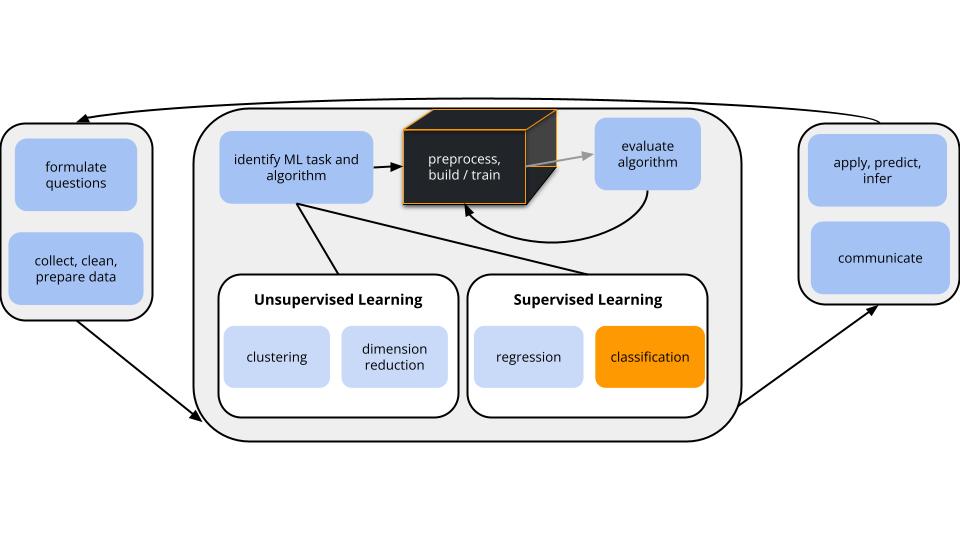
CONTEXT
world = supervised learning
We want to model some output variable \(y\) using a set of potential predictors (\(x_1, x_2, ..., x_p\)).
task = CLASSIFICATION
\(y\) is categorical
algorithm = NONparametric
GOAL
Build and evaluate nonparametric classification models of some categorical outcome y.
How do we evaluate classification models?
. . .
Binary Metrics:
. . .
More Binary Metrics [optional]:
. . .
Multiclass Metrics:
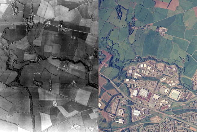
We’ll continue to classify land type using metrics from aerial photographs:
# Load & process data
# NOTE: Our y variable has to be converted to a "factor" variable, not a character string
land <- read.csv("https://Mac-Stat.github.io/data/land_cover.csv") %>%
rename(type = class) %>%
mutate(type = as.factor(type))# There are 9 land types!
# Let's consider all of them (not just asphalt, grass, trees)
land %>%
count(type) type n
1 asphalt 59
2 building 122
3 car 36
4 concrete 116
5 grass 112
6 pool 29
7 shadow 61
8 soil 34
9 tree 106# There are 675 data points and 147 potential predictors of land type!
dim(land)[1] 675 148# For now: we'll consider Mean_G & NDVI
# (It's not easy to visually distinguish between 9 colors!)
# Plot type vs Mean_G alone
ggplot(land, aes(x = Mean_G, fill = type)) +
geom_density(alpha = 0.5) +
scale_fill_manual(values = c("#000000", "darkgray", "red", "#7570B3", "lightgreen", "blue", "#E6AB02", "brown", "#66A61E")) +
theme_minimal()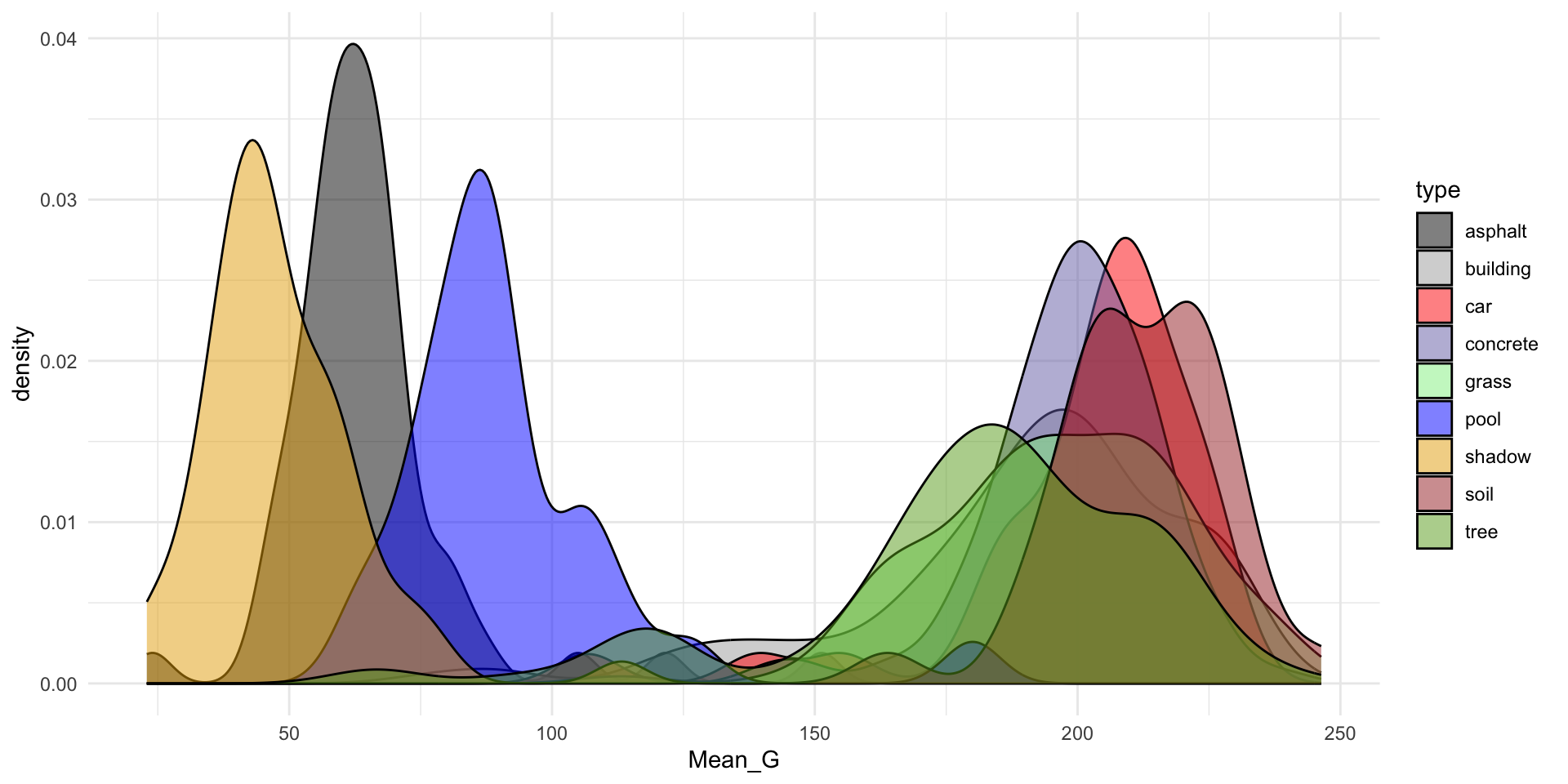
# Plot type vs NDVI alone
ggplot(land, aes(x = NDVI, fill = type)) +
  geom_density(alpha = 0.5) +
  scale_fill_manual(values = c("#000000", "darkgray", "red", "#7570B3", "lightgreen", "blue", "#E6AB02", "brown", "#66A61E")) +
  theme_minimal()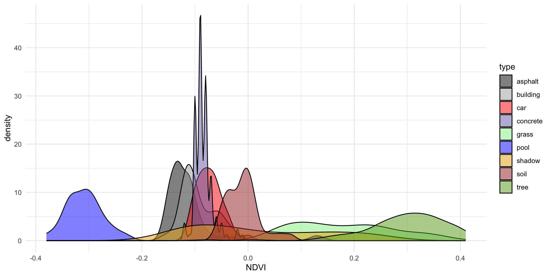
# Finally consider both
ggplot(land, aes(y = Mean_G, x = NDVI, color = type)) +
  geom_point() +
  scale_color_manual(values = c("#000000", "darkgray", "red", "#7570B3", "lightgreen", "blue", "#E6AB02", "brown", "#66A61E")) +
  theme_minimal()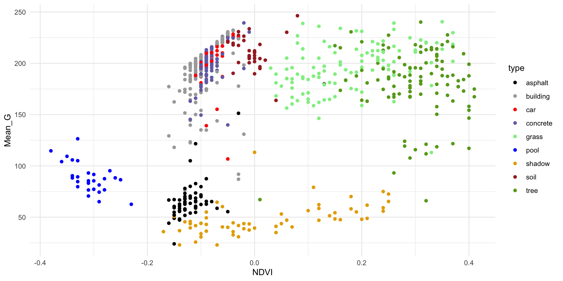
Discuss the following examples with your group.
Check out the classification regions for two KNN models of land type by Mean_G and NDVI: using K = 1 neighbor and using K = 16 neighbors.
Though the KNN models were built using standardized predictors, the predictors are plotted on their original scales here.
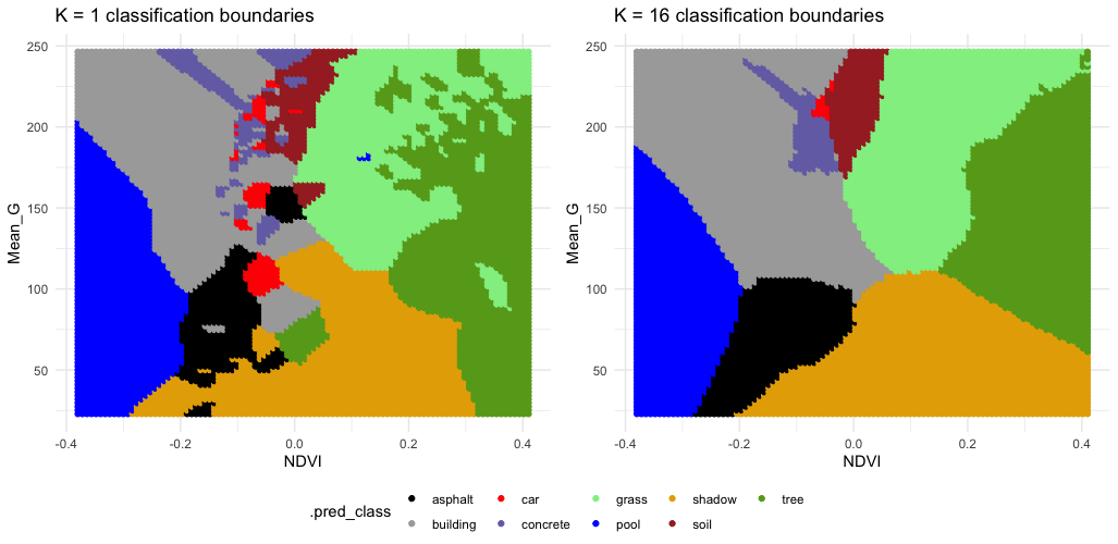
Discuss:
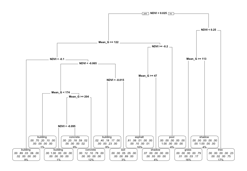
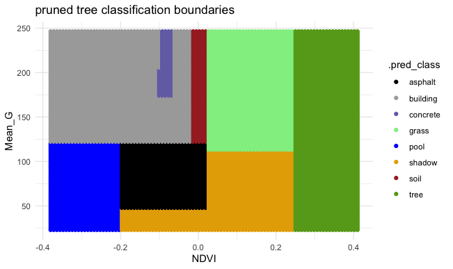
Next, consider a PRUNED classification tree of land type by Mean_G and NDVI that was pruned as follows:
Discuss:
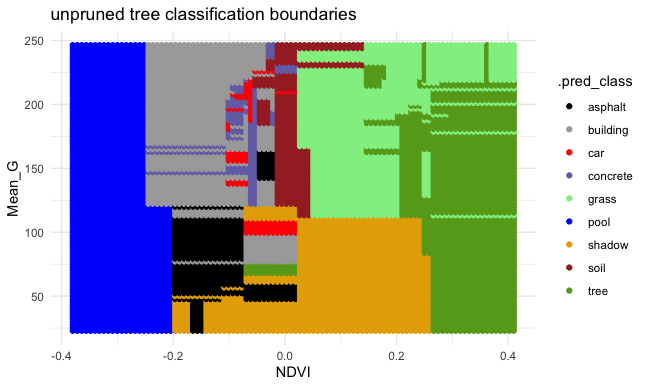
Finally, consider a (mostly) UNPRUNED classification tree of land type by Mean_G and NDVI that was built using the following tuning parameters:
Check out the classification regions defined by this tree:
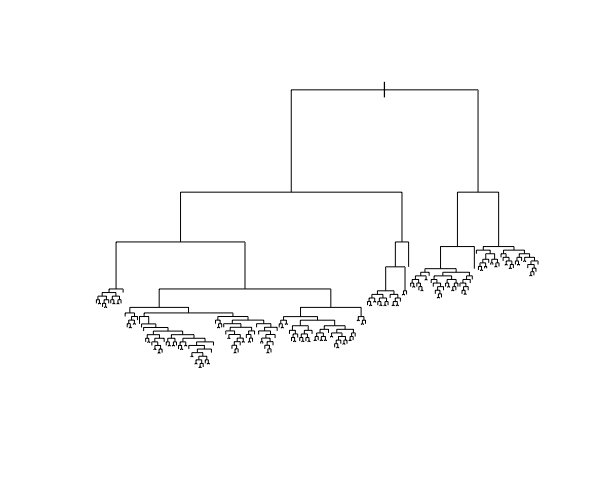
And the tree itself.
This tree was plotted using a function that draws the length of each branch split to be proportional to its improvement to the classification accuracy. The labels are left off to just focus on structure:
Discuss:
Gini Index: Node Purity Measure
\[G = p_1(1-p_1) + p_2(1-p_2) + \cdots + p_k(1-p_k)\]
Information/Entropy Index: Alternative to Gini
\[I = -(p_1\log(p_1) + p_2\log(p_2) + \cdots + p_k\log(p_k))\]
Let’s focus on trees.
We’ve explored some general ML themes already:
model building: parametric vs nonparametric
benefits and drawbacks of using nonparametric trees vs parametric algorithm logistic regression
algorithm details:
In the exercises, you’ll explore some other important themes:
model building: variable selection
We have 147 potential predictors of land type. How can we choose which ones to use?
model evaluation & comparison
How good are our trees? Which one should we pick?
regression vs classification
KNN works in both settings. So do trees!
In modeling land type by all 147 possible predictors, our goal will be to build a tree that optimize the cost_complexity parameter. The chunk below builds 10 trees, each using a different cost_complexity value while fixing our other tuning parameters to be very liberal / not restrictive:
tree_depth = 30 (the default)min_n in each leaf node = 2 (the default is 20)Reflect on the code and pause to answer any questions (Q).
# STEP 1: tree specification
# Q: WHAT IS NEW HERE?!
tree_spec <- decision_tree() %>%
  set_mode("classification") %>%
  set_engine(engine = "rpart") %>%
  set_args(cost_complexity = tune(),
           min_n = 2,
           tree_depth = NULL)
# STEP 2: variable recipe
# NOTHING IS NEW HERE & THERE ARE NO PREPROCESSING STEPS!
variable_recipe_big <- recipe(type ~ ., data = land)
# STEP 3: tree workflow
# NOTHING IS NEW HERE!
tree_workflow_big <- workflow() %>%
add_recipe(variable_recipe_big) %>%
add_model(tree_spec)# STEP 4: Estimate 10 trees using a range of possible cost complexity values
# cost_complexity is on the log10 scale (10^(-5) to 10^(0.1))
# Q: BY WHAT CV METRIC ARE WE COMPARING THE TREES?
# Q: WHY NOT USE CV MAE?
set.seed(253)
tree_models_big <- tree_workflow_big %>%
tune_grid(
grid = grid_regular(cost_complexity(range = c(-5, 0.1)), levels = 10),
resamples = vfold_cv(land, v = 10),
metrics = metric_set(accuracy)
)
We only built 10 trees above, and it took quite a bit of time. Why are trees computationally expensive?
Just as with our other algorithms with tuning parameters, we can use the CV metrics to compare the 10 trees, and pick which one we prefer.
Here, we’ll pick the parsimonious tree (which also happens to be the tree with the largest CV accuracy!).
Run & reflect upon the code below, then answer some follow-up questions.
# Compare the CV metrics for the 10 trees
tree_models_big %>%
  autoplot() +
  scale_x_continuous()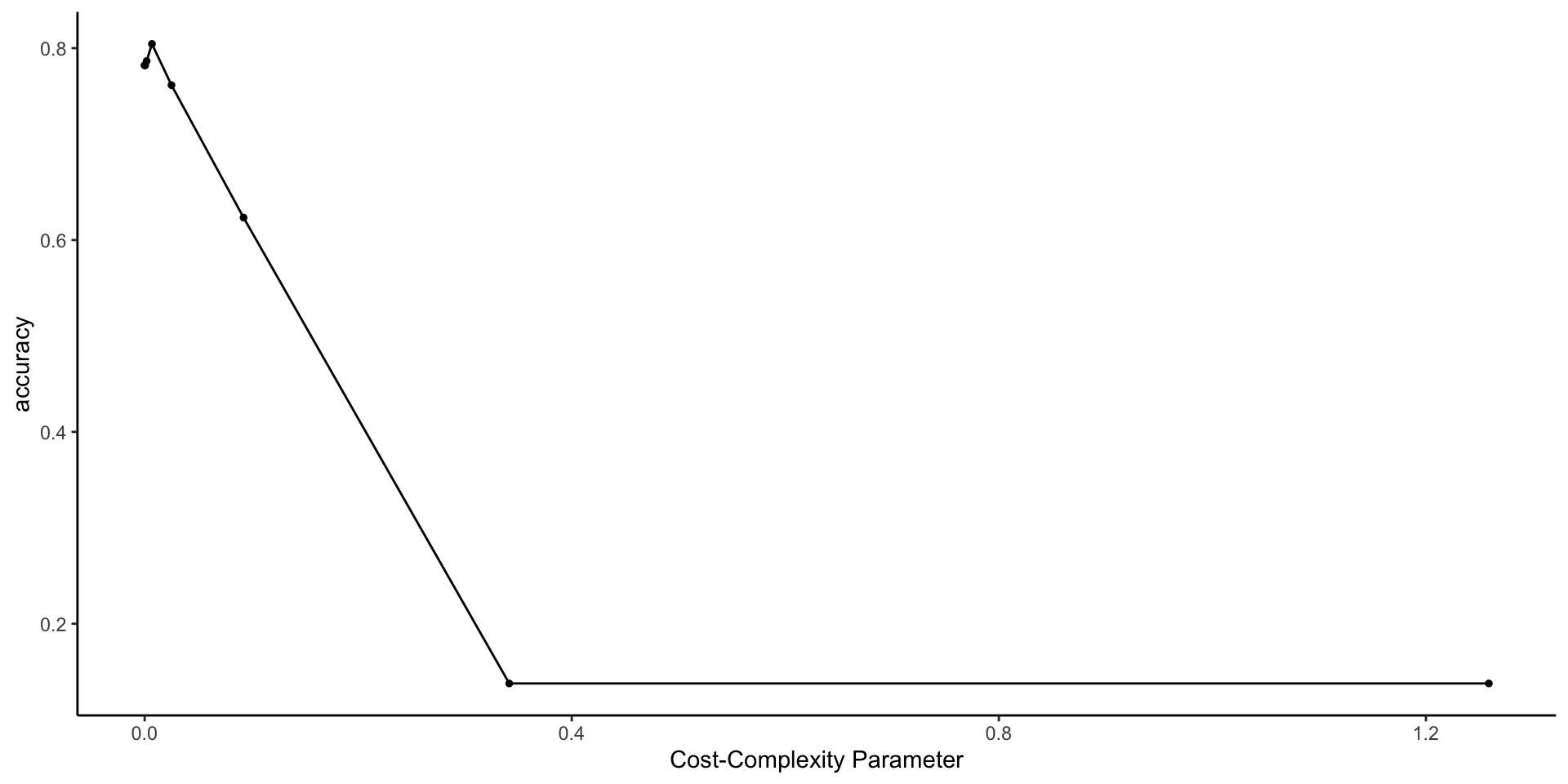
# Pick the parsimonious parameter
parsimonious_param_big <- tree_models_big %>%
  select_by_one_std_err(metric = "accuracy", desc(cost_complexity))
parsimonious_param_big
# A tibble: 1 × 2
cost_complexity .config
<dbl> <chr>
1 0.00681 Preprocessor1_Model06# Finalize the tree with parsimonious cost complexity
big_tree <- tree_workflow_big %>%
finalize_workflow(parameters = parsimonious_param_big) %>%
fit(data = land)
Let’s examine the final, tuned big_tree which models land type by all 147 predictors:
# This tree has a bunch of info
# BUT: (1) it's tough to read; and (2) all branch lengths are the same (not proportional to their improvement)
big_tree %>%
  extract_fit_engine() %>%
  rpart.plot()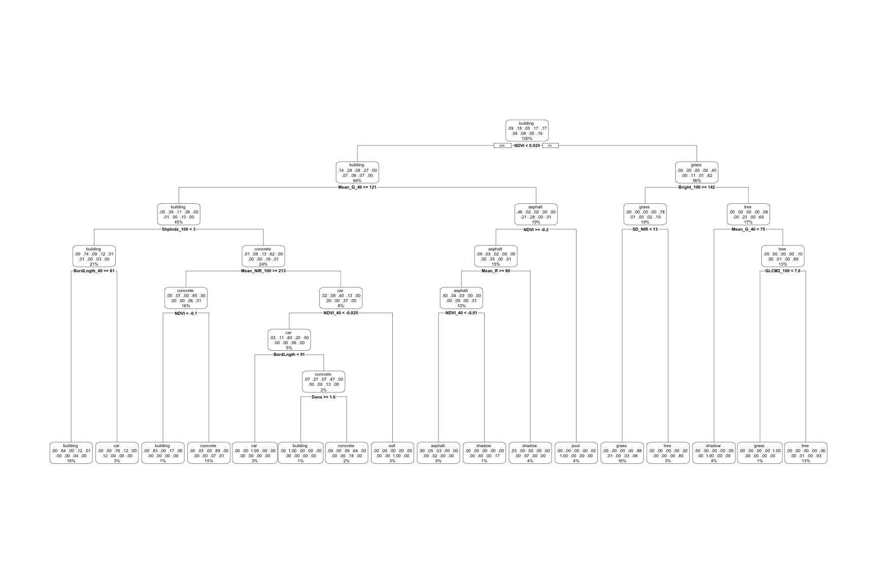
# We can make it a little easier by playing around with
# font size (cex) and removing some node details (type = 0)
big_tree %>%
  extract_fit_engine() %>%
  rpart.plot(cex = 0.8, type = 0)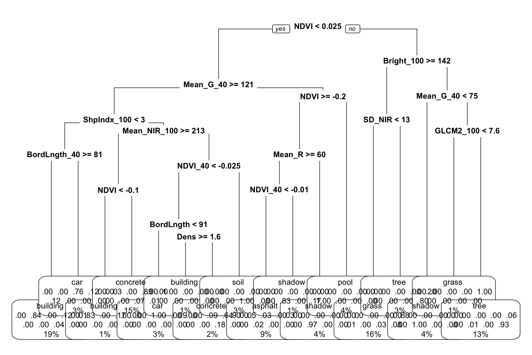
# This tree (1) is easier to read; and (2) plots branch lengths proportional to their improvement
# But it has less info about classification accuracy
big_tree %>%
  extract_fit_engine() %>%
  plot()
big_tree %>%
  extract_fit_engine() %>%
  text(cex = 0.8)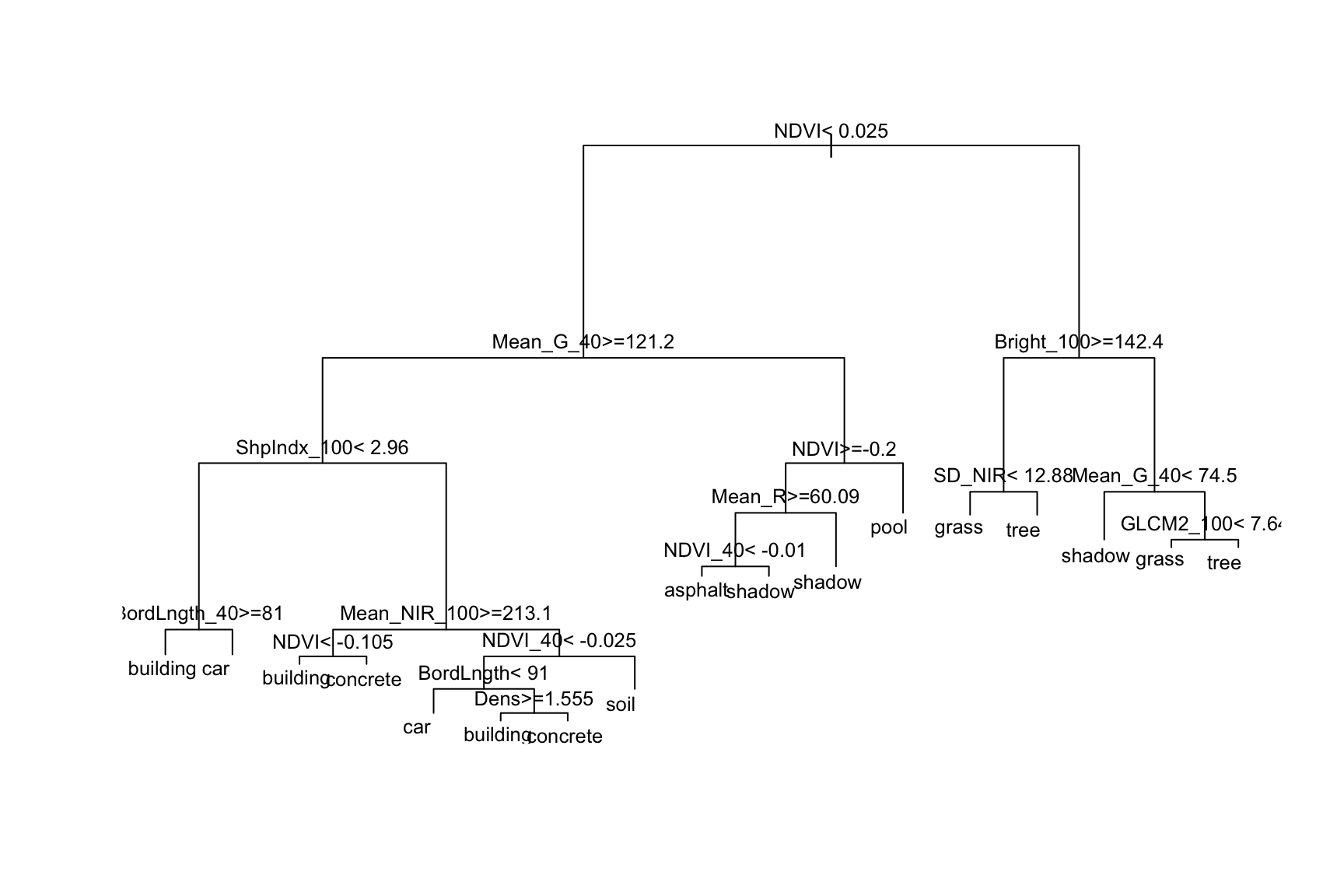
Use the second tree plot to answer the following questions.
Luckily, we don’t have to guesstimate the importance of different predictors.
There’s a mathematical metric: variable importance.
Roughly, a predictor’s importance measures the total improvement in node purity if we were to split on this predictor (even if the predictor isn’t ultimately used in a split).
The bigger the better!
Check out the importance of our 147 predictors.
# Check out just the 10 most important (for simplicity)
big_tree %>%
  extract_fit_engine() %>%
  pluck("variable.importance") %>%
  head(10)
NDVI_40 NDVI NDVI_60 Mean_G Bright_40 Mean_G_40
140.81912 136.74372 128.66465 117.47329 110.15678 95.89161
NDVI_80 NDVI_100 NDVI_120 Mean_NIR_100
84.91799 76.13970 71.44863 70.28818 And plot these to help with comparison:
# By default, this plots only 10 predictors
# At most, it will plot only half of our predictors here
# (I'm not sure what the max is in general!)
library(vip)
big_tree %>%
  vip(geom = "point", num_features = 147)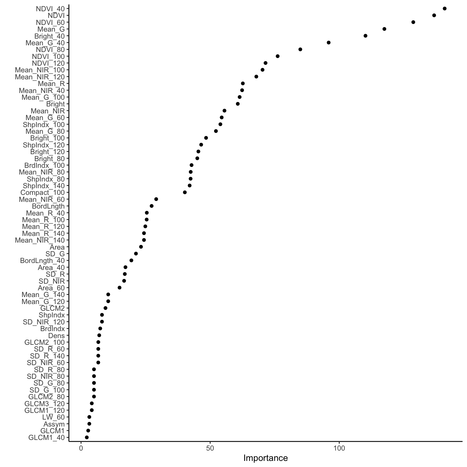
Stepping back, our goal for building this tree was to classify land type for a pixel in an image.
As an example, suppose we have a pixel in an image like the first one in our data set:
head(land, 1) type BrdIndx Area Round Bright Compact ShpIndx Mean_G Mean_R Mean_NIR SD_G
1 car 1.27 91 0.97 231.38 1.39 1.47 207.92 241.74 244.48 21.41
SD_R SD_NIR LW GLCM1 Rect GLCM2 Dens Assym NDVI BordLngth GLCM3
1 20.4 18.69 2.19 0.48 0.87 6.23 1.6 0.74 -0.08 56 4219.69
BrdIndx_40 Area_40 Round_40 Bright_40 Compact_40 ShpIndx_40 Mean_G_40
1 1.33 97 1.12 227.19 1.32 1.42 203.95
Mean_R_40 Mean_NIR_40 SD_G_40 SD_R_40 SD_NIR_40 LW_40 GLCM1_40 Rect_40
1 237.23 240.38 27.63 28.36 26.18 2 0.5 0.85
GLCM2_40 Dens_40 Assym_40 NDVI_40 BordLngth_40 GLCM3_40 BrdIndx_60 Area_60
1 6.29 1.67 0.7 -0.08 56 3806.36 1.33 97
Round_60 Bright_60 Compact_60 ShpIndx_60 Mean_G_60 Mean_R_60 Mean_NIR_60
1 1.12 227.19 1.32 1.42 203.95 237.23 240.38
SD_G_60 SD_R_60 SD_NIR_60 LW_60 GLCM1_60 Rect_60 GLCM2_60 Dens_60 Assym_60
1 27.63 28.36 26.18 2 0.5 0.85 6.29 1.67 0.7
NDVI_60 BordLngth_60 GLCM3_60 BrdIndx_80 Area_80 Round_80 Bright_80
1 -0.08 56 3806.36 1.33 97 1.12 227.19
Compact_80 ShpIndx_80 Mean_G_80 Mean_R_80 Mean_NIR_80 SD_G_80 SD_R_80
1 1.32 1.42 203.95 237.23 240.38 27.63 28.36
SD_NIR_80 LW_80 GLCM1_80 Rect_80 GLCM2_80 Dens_80 Assym_80 NDVI_80
1 26.18 2 0.5 0.85 6.29 1.67 0.7 -0.08
BordLngth_80 GLCM3_80 BrdIndx_100 Area_100 Round_100 Bright_100 Compact_100
1 56 3806.36 1.33 97 1.12 227.19 1.32
ShpIndx_100 Mean_G_100 Mean_R_100 Mean_NIR_100 SD_G_100 SD_R_100 SD_NIR_100
1 1.42 203.95 237.23 240.38 27.63 28.36 26.18
LW_100 GLCM1_100 Rect_100 GLCM2_100 Dens_100 Assym_100 NDVI_100 BordLngth_100
1 2 0.5 0.85 6.29 1.67 0.7 -0.08 56
GLCM3_100 BrdIndx_120 Area_120 Round_120 Bright_120 Compact_120 ShpIndx_120
1 3806.36 1.33 97 1.12 227.19 1.32 1.42
Mean_G_120 Mean_R_120 Mean_NIR_120 SD_G_120 SD_R_120 SD_NIR_120 LW_120
1 203.95 237.23 240.38 27.63 28.36 26.18 2
GLCM1_120 Rect_120 GLCM2_120 Dens_120 Assym_120 NDVI_120 BordLngth_120
1 0.5 0.85 6.29 1.67 0.7 -0.08 56
GLCM3_120 BrdIndx_140 Area_140 Round_140 Bright_140 Compact_140 ShpIndx_140
1 3806.36 1.33 97 1.12 227.19 1.32 1.42
Mean_G_140 Mean_R_140 Mean_NIR_140 SD_G_140 SD_R_140 SD_NIR_140 LW_140
1 203.95 237.23 240.38 27.63 28.36 26.18 2
GLCM1_140 Rect_140 GLCM2_140 Dens_140 Assym_140 NDVI_140 BordLngth_140
1 0.5 0.85 6.29 1.67 0.7 -0.08 56
GLCM3_140
1 3806.36Our tree correctly predicts that this is a car:
big_tree %>%
  predict(new_data = head(land, 1))
# A tibble: 1 × 1
.pred_class
<fct>
1 "car " But how good are the classifications overall?
Let’s first consider the CV overall accuracy rate:
# reminder of our chosen tuning parameter
parsimonious_param_big
# A tibble: 1 × 2
cost_complexity .config
<dbl> <chr>
1 0.00681 Preprocessor1_Model06# pull out metrics for just that value of tuning parameter
tree_models_big %>%
collect_metrics() %>%
filter(cost_complexity == parsimonious_param_big$cost_complexity)# A tibble: 1 × 7
cost_complexity .metric .estimator mean n std_err .config
<dbl> <chr> <chr> <dbl> <int> <dbl> <chr>
1 0.00681 accuracy multiclass 0.804 10 0.0172 Preprocessor1_Model06Interpret 0.804, the CV overall accuracy rate for the big_tree.
Calculate & compare the tree’s CV overall accuracy rate to the no information rate: is the big_tree better than just always guessing the most common land type? You’ll need the following info:
land %>%
  nrow()
[1] 675land %>%
count(type) type n
1 asphalt 59
2 building 122
3 car 36
4 concrete 116
5 grass 112
6 pool 29
7 shadow 61
8 soil 34
9 tree 106
The above CV metric gives us a sense of the overall quality of using our tree to classify a new pixel in an image.
But it doesn’t give any insight into the quality of classifications for any particular land type.
To that end, let’s consider the in-sample confusion matrix (i.e. how well our tree classified the pixels in an image in our sample).
NOTE: We could also get a CV version, but the code is long and the CV accuracy will do for now!
in_sample_confusion <- big_tree %>%
  augment(new_data = land) %>%
  conf_mat(truth = type, estimate = .pred_class)

in_sample_confusion
Truth
Prediction asphalt building car concrete grass pool shadow soil tree
asphalt 57 3 2 0 0 0 1 0 0
building 0 116 0 16 1 0 0 5 0
car 0 0 33 2 0 2 0 0 0
concrete 1 3 1 98 0 0 0 9 1
grass 0 0 0 0 102 1 0 3 9
pool 0 0 0 0 0 26 0 0 0
shadow 1 0 0 0 0 0 59 0 1
soil 0 0 0 0 0 0 0 17 0
tree 0 0 0 0 9 0 1 0 95# The mosaic plot of this matrix is too messy to be very useful here
in_sample_confusion %>%
autoplot() +
aes(fill = rep(colnames(in_sample_confusion$table), ncol(in_sample_confusion$table))) +
scale_fill_manual(values = c("#000000", "darkgray", "red", "#7570B3", "lightgreen", "blue", "#E6AB02", "brown", "#66A61E")) +
theme(legend.position = "none")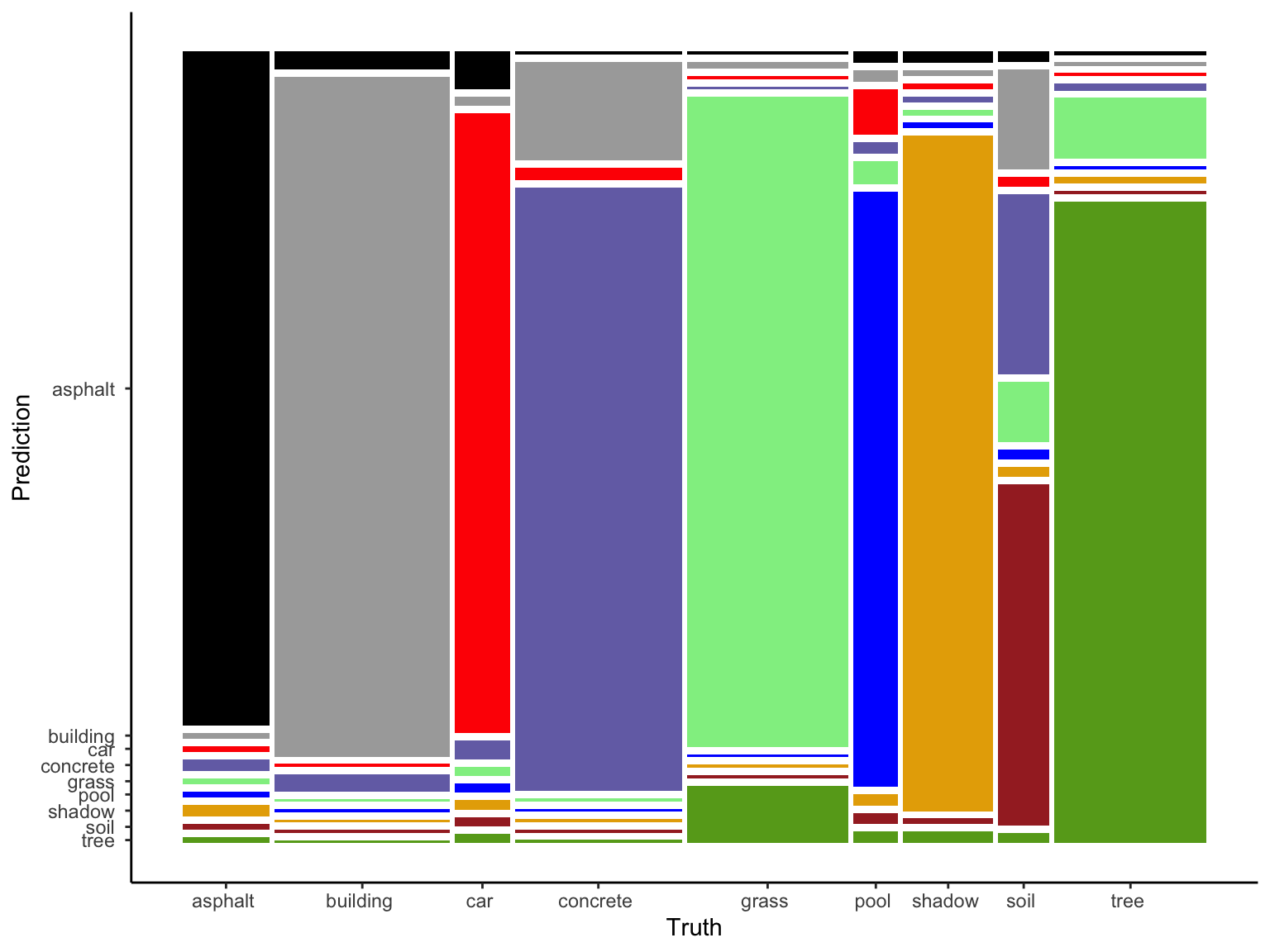
Just like KNN, trees can be applied in both regression and classification settings.
Thus trees add to our collection of nonparametric regression techniques, including KNN, LOESS, and GAM.
To explore, we’ll use regression trees to model the body_mass_g of penguins by their bill_length_mm and species. This is for demonstration purposes only!!!
As the plot below demonstrates, this relationship isn’t complicated enough to justify using a nonparametric algorithm:
data(penguins)
ggplot(penguins, aes(y = body_mass_g, x = bill_length_mm, color = species)) +
  geom_point()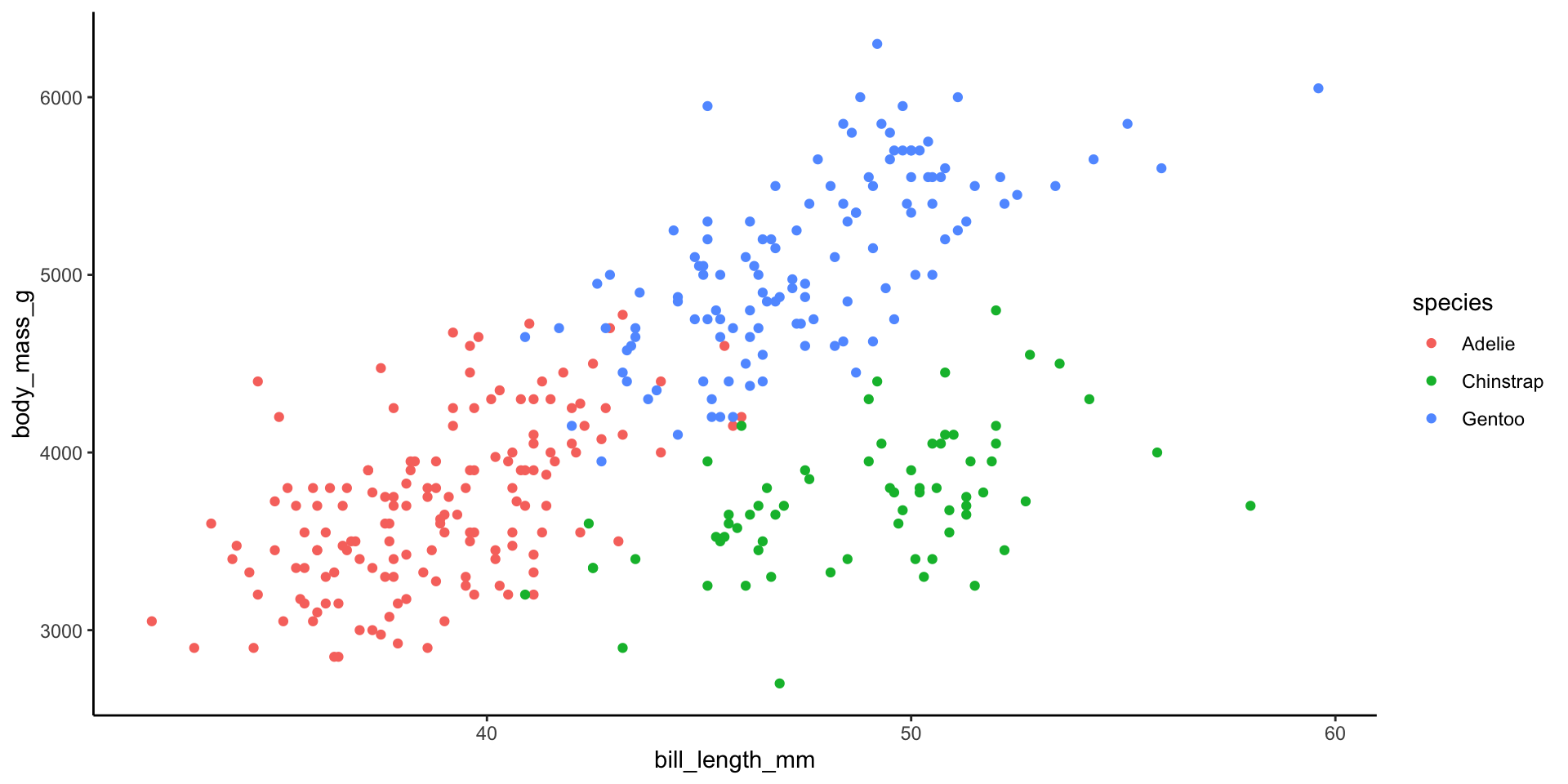
Run the following code to build a regression tree of this relationship.
Pause to reflect upon the questions in the comments:
# CHUNK GOAL
# Build a bunch of trees using different cost complexity parameters

# STEP 1: regression tree specification
# QUESTION: How does this differ from our classification tree specification?
tree_spec <- decision_tree() %>%
  set_mode("regression") %>%
  set_engine(engine = "rpart") %>%
  set_args(cost_complexity = tune(),
           min_n = 2,
           tree_depth = 20)

# STEP 2: variable recipe
# NOTHING IS NEW HERE!
variable_recipe <- recipe(body_mass_g ~ bill_length_mm + species, data = penguins)

# STEP 3: tree workflow
# NOTHING IS NEW HERE!
tree_workflow <- workflow() %>%
  add_recipe(variable_recipe) %>%
  add_model(tree_spec)

# STEP 4: Estimate multiple trees using a range of possible cost complexity values
# QUESTION: How do the CV metrics differ from our classification tree?
set.seed(253)
tree_models <- tree_workflow %>%
  tune_grid(
    grid = grid_regular(cost_complexity(range = c(-5, -1)), levels = 10),
    resamples = vfold_cv(penguins, v = 10),
    metrics = metric_set(mae)
  )
# CHUNK GOAL:
# Finalize the tree using the parsimonious cost complexity parameter
# NOTHING IS NEW HERE
# Identify the parsimonious cost complexity parameter
parsimonious_param <- tree_models %>%
select_by_one_std_err(metric = "mae", desc(cost_complexity))
# Finalize the tree with parsimonious cost complexity
regression_tree <- tree_workflow %>%
finalize_workflow(parameters = parsimonious_param) %>%
fit(data = penguins)
Check out the resulting regression tree:
# This code is the same as for classification trees!
regression_tree %>%
  extract_fit_engine() %>%
  rpart.plot()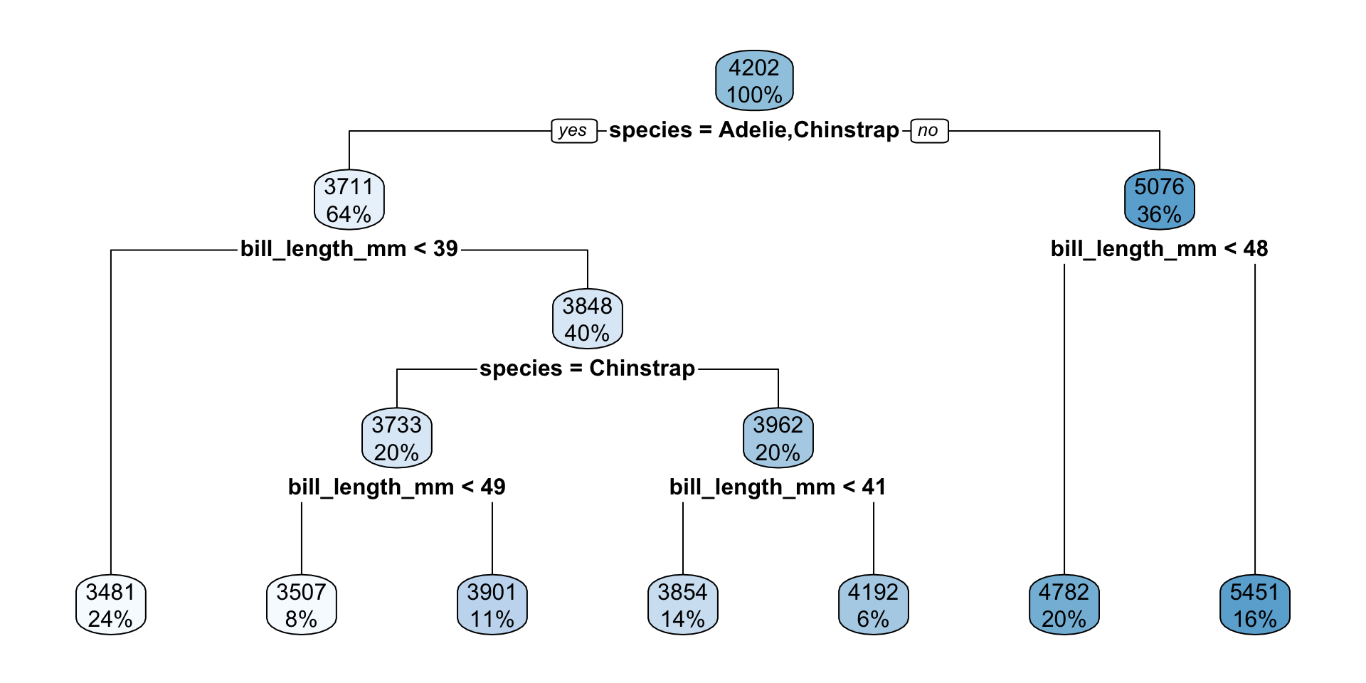
new_penguins <- data.frame(species = c("Adelie", "Gentoo"), bill_length_mm = c(45, 45))
new_penguins
species bill_length_mm
1 Adelie 45
2 Gentoo 45regression_tree %>%
augment(new_data = new_penguins)# A tibble: 2 × 3
.pred species bill_length_mm
<dbl> <chr> <dbl>
1 4192. Adelie 45
2 4782. Gentoo 45regression_tree %>%
augment(new_data = penguins) %>%
ggplot(aes(x = bill_length_mm, y = body_mass_g, color = species)) +
geom_point(alpha = 0.35, size = 0.5) +
geom_point(aes(x = bill_length_mm, y = .pred, color = species), size = 1.5) +
facet_wrap(~ species) +
theme_minimal()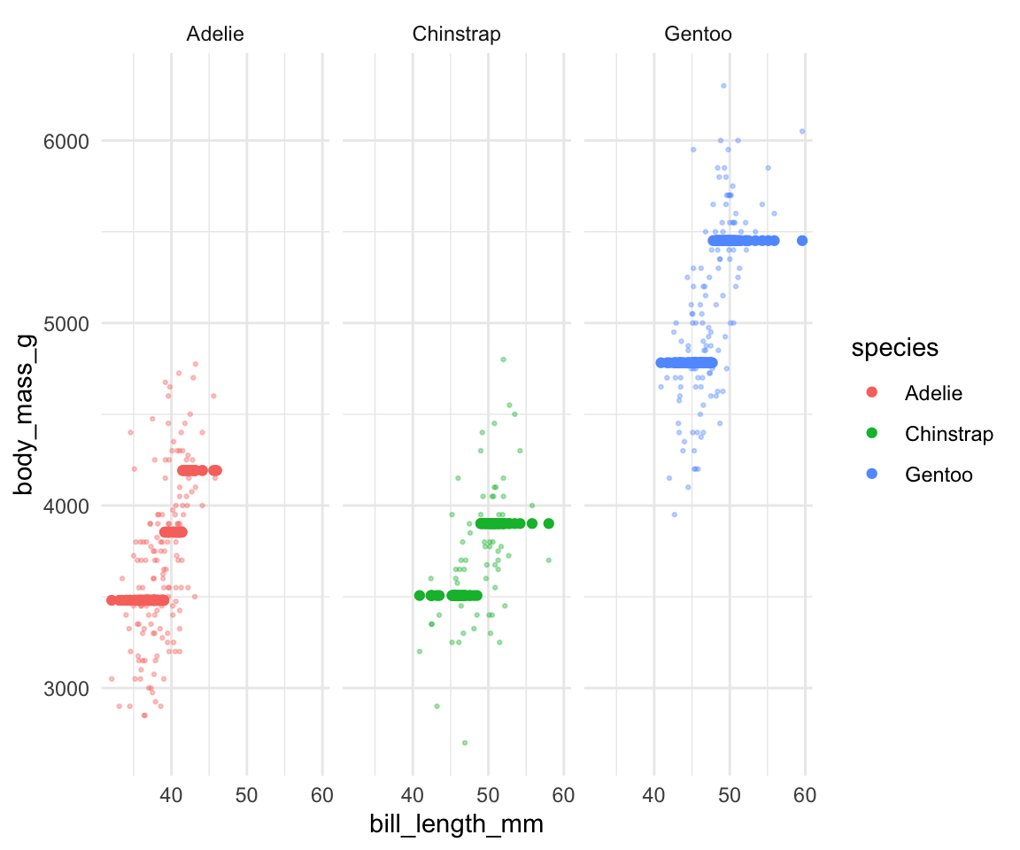
Check out this visual essay on trees!
With your remaining time, work on HW5.
Suppose we want to build a KNN model of some categorical response variable y using predictors x1 and x2 in our sample_data.
# Load packages
library(tidymodels)
library(kknn)

# Resolves package conflicts by preferring tidymodels functions
tidymodels_prefer()
Make sure that y is a factor variable
sample_data <- sample_data %>%
  mutate(y = as.factor(y))
Build models for a variety of tuning parameters K
# STEP 1: KNN model specification
knn_spec <- nearest_neighbor() %>%
  set_mode("classification") %>%
  set_engine(engine = "kknn") %>%
  set_args(neighbors = tune())

# STEP 2: variable recipe
variable_recipe <- recipe(y ~ x1 + x2, data = sample_data) %>%
  step_nzv(all_predictors()) %>%
  step_dummy(all_nominal_predictors()) %>%
  step_normalize(all_numeric_predictors())

# STEP 3: KNN workflow
knn_workflow <- workflow() %>%
  add_recipe(variable_recipe) %>%
  add_model(knn_spec)

# STEP 4: Estimate multiple KNN models using a range of possible K values
set.seed(___)
knn_models <- knn_workflow %>%
  tune_grid(
    grid = grid_regular(neighbors(range = c(___, ___)), levels = ___),
    resamples = vfold_cv(sample_data, v = ___),
    metrics = metric_set(accuracy)
  )
Tuning K
# Calculate CV accuracy for each KNN model
knn_models %>%
  collect_metrics()

# Plot CV accuracy (y-axis) for the KNN model from each K (x-axis)
knn_models %>%
  autoplot()

# Identify K which produced the highest (best) CV accuracy
best_K <- select_best(knn_models, metric = "accuracy")
best_K

# Get the CV accuracy for KNN when using best_K
knn_models %>%
  collect_metrics() %>%
  filter(neighbors == best_K$neighbors)
Finalizing the “best” KNN model
final_knn_model <- knn_workflow %>%
  finalize_workflow(parameters = best_k) %>%
  fit(data = sample_data)
Use the KNN to make predictions / classifications
# Put in a data.frame object with x1 and x2 values (at minimum)
final_knn_model %>%
  predict(new_data = ___)
Suppose we want to build a tree of some categorical response variable y using predictors x1 and x2 in our sample_data.
# Load packages
library(tidymodels)
library(rpart)
library(rpart.plot)

# Resolves package conflicts by preferring tidymodels functions
tidymodels_prefer()
Make sure that y is a factor variable
sample_data <- sample_data %>%
  mutate(y = as.factor(y))
Build trees for a variety of tuning parameters
We’ll focus on optimizing the cost_complexity parameter, while setting min_n and tree_depth to fixed numbers. For example, setting min_n to 2 and tree_depth to 30 set only loose restrictions, letting cost_complexity do the pruning work.
# STEP 1: tree specification
# If y is quantitative, change "classification" to "regression"
tree_spec <- decision_tree() %>%
  set_mode("classification") %>%
  set_engine(engine = "rpart") %>%
  set_args(cost_complexity = tune(),
           min_n = 2,
           tree_depth = 30)

# STEP 2: variable recipe
# There are no necessary preprocessing steps for trees!
variable_recipe <- recipe(y ~ x1 + x2, data = sample_data)

# STEP 3: tree workflow
tree_workflow <- workflow() %>%
  add_recipe(variable_recipe) %>%
  add_model(tree_spec)

# STEP 4: Estimate multiple trees using a range of possible cost complexity values
# - If y is quantitative, change "accuracy" to "mae"
# - cost_complexity is on the log10 scale (10^(-5) to 10^(0.1))
#   I start with a range from -5 to 2 and then tweak
set.seed(___)
tree_models <- tree_workflow %>%
  tune_grid(
    grid = grid_regular(cost_complexity(range = c(___, ___)), levels = ___),
    resamples = vfold_cv(sample_data, v = ___),
    metrics = metric_set(accuracy)
  )
Tuning cost complexity
# Plot the CV accuracy vs cost complexity for our trees
# x-axis is on the original (not log10) scale
tree_models %>%
  autoplot() +
  scale_x_continuous()

# Identify cost complexity which produced the highest CV accuracy
best_cost <- tree_models %>%
  select_best(metric = "accuracy")

# Get the CV accuracy when using best_cost
tree_models %>%
  collect_metrics() %>%
  filter(cost_complexity == best_cost$cost_complexity)

# Identify cost complexity which produced the parsimonious tree
parsimonious_cost <- tree_models %>%
  select_by_one_std_err(metric = "accuracy", desc(cost_complexity))
Finalizing the tree
# Plug in best_cost or parsimonious_cost
final_tree <- tree_workflow %>%
  finalize_workflow(parameters = ___) %>%
  fit(data = sample_data)
Plot the tree
# Tree with accuracy info in each node
# Branches are NOT proportional to classification improvement
final_tree %>%
  extract_fit_engine() %>%
  rpart.plot()

# Tree withOUT accuracy info in each node
# Branches ARE proportional to classification improvement
final_tree %>%
  extract_fit_engine() %>%
  plot()
final_tree %>%
  extract_fit_engine() %>%
  text()
Use the tree to make predictions / classifications
# Put in a data.frame object with x1 and x2 values (at minimum)
final_tree %>%
  predict(new_data = ___)

# OR
final_tree %>%
  augment(new_data = ___)
Examine variable importance
# Print the metrics
final_tree %>%
  extract_fit_engine() %>%
  pluck("variable.importance")

# Plot the metrics
# Plug in the number of top predictors you wish to plot
# (The upper limit varies by application!)
library(vip)
final_tree %>%
  vip(geom = "point", num_features = ___)
Evaluate the classifications using in-sample metrics
# Get the in-sample confusion matrix
in_sample_confusion <- final_tree %>%
  augment(new_data = sample_data) %>%
  conf_mat(truth = type, estimate = .pred_class)
in_sample_confusion

# Plot the matrix using a mosaic plot
# See exercise for what to do when there are more categories than colors in our pallette!
in_sample_confusion %>%
  autoplot() +
  aes(fill = rep(colnames(in_sample_confusion$table), ncol(in_sample_confusion$table))) +
  theme(legend.position = "none")
Example 1: KNN
Example 2: Pruned tree
Example 3: Unpruned tree
Exercise 1: Build 10 trees
See comments below.
# STEP 1: tree specification
# Q: WHAT IS NEW HERE?!
tree_spec <- decision_tree() %>% # decision_tree() is new
  set_mode("classification") %>% # still in the classification mode!
  set_engine(engine = "rpart") %>% # new engine (rpart) for trees
  set_args(cost_complexity = tune(),  # new arguments for trees
           min_n = 2,
           tree_depth = NULL)
# STEP 2: variable recipe
# NOTHING IS NEW HERE & THERE ARE NO PREPROCESSING STEPS!
variable_recipe_big <- recipe(type ~ ., data = land)
# STEP 3: tree workflow
# NOTHING IS NEW HERE!
tree_workflow_big <- workflow() %>%
add_recipe(variable_recipe_big) %>%
add_model(tree_spec)# STEP 4: Estimate 10 trees using a range of possible cost complexity values
# cost_complexity is on the log10 scale (10^(-5) to 10^(0.1))
# Q: BY WHAT CV METRIC ARE WE COMPARING THE TREES?
# Q: WHY NOT USE CV MAE?
set.seed(253)
tree_models_big <- tree_workflow_big %>%
tune_grid(
grid = grid_regular(cost_complexity(range = c(-5, 0.1)), levels = 10),
resamples = vfold_cv(land, v = 10),
metrics = metric_set(accuracy) # use accuracy instead of MAE since this is classification not regression
)Exercise 2: Whew!
Exercise 3: Compare and finalize the tree
Exercise 4: Examine the tree
Exercise 5: Identifying useful predictors
Exercise 6: How good is the tree?!? Part 1
big_tree will correctly classify roughly 80% of new pixel in an image.122/675 [1] 0.1807407Exercise 7: How good is the tree?!? Part 2
Part 2 Setup
data(penguins)
ggplot(penguins, aes(y = body_mass_g, x = bill_length_mm, color = species)) +
  geom_point()
# CHUNK GOAL
# Build a bunch of trees using different cost complexity parameters

# STEP 1: regression tree specification
# QUESTION: How does this differ from our classification tree specification?
tree_spec <- decision_tree() %>%
  set_mode("regression") %>% # ANSWER: switch to regression mode!
  set_engine(engine = "rpart") %>%
  set_args(cost_complexity = tune(),
           min_n = 2,
           tree_depth = 20)

# STEP 2: variable recipe
# NOTHING IS NEW HERE!
variable_recipe <- recipe(body_mass_g ~ bill_length_mm + species, data = penguins)

# STEP 3: tree workflow
# NOTHING IS NEW HERE!
tree_workflow <- workflow() %>%
  add_recipe(variable_recipe) %>%
  add_model(tree_spec)

# STEP 4: Estimate multiple trees using a range of possible cost complexity values
# QUESTION: How do the CV metrics differ from our classification tree?
set.seed(253)
tree_models <- tree_workflow %>%
  tune_grid(
    grid = grid_regular(cost_complexity(range = c(-5, -1)), levels = 10),
    resamples = vfold_cv(penguins, v = 10),
    metrics = metric_set(mae) # ANSWER: switch to MAE
  )
# CHUNK GOAL:
# Finalize the tree using the parsimonious cost complexity parameter
# NOTHING IS NEW HERE
# Identify the parsimonious cost complexity parameter
parsimonious_param <- tree_models %>%
select_by_one_std_err(metric = "mae", desc(cost_complexity))
# Finalize the tree with parsimonious cost complexity
regression_tree <- tree_workflow %>%
finalize_workflow(parameters = parsimonious_param) %>%
fit(data = penguins)Exercise 8: Regression tree
Exercise 9: Visual essay
Exercise 10: Work on Homework