Topic 14 Bagging and Random Forests
Learning Goals
- Explain the rationale for bagging
- Explain the rationale for selecting a random subset of predictors at each split (random forests)
- Explain how the size of the random subset of predictors at each split relates to the bias-variance tradeoff
- Explain the rationale for and implement out-of-bag error estimation for both regression and classification
- Explain the rationale behind the random forest variable importance measure and why it is biased towards quantitative predictors
Slides from today are available here.
Exercises
You can download a template RMarkdown file to start from here.
Before proceeding, install the ranger and vip package by entering install.packages("ranger","vip") in the Console.
Our goal will be to classify types of urban land cover in small subregions within a high resolution aerial image of a land region. Data from the UCI Machine Learning Repository include the observed type of land cover (determined by human eye) and “spectral, size, shape, and texture information” computed from the image. See this page for the data codebook.
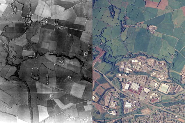
Source: https://ncap.org.uk/sites/default/files/EK_land_use_0.jpg
library(dplyr)
library(readr)
library(ggplot2)
library(vip)
library(tidymodels)
tidymodels_prefer()
conflicted::conflict_prefer("vi", "vip")

# Read in the data
land <- read_csv("https://www.macalester.edu/~ajohns24/data/land_cover.csv")

# There are 9 land types, but we'll focus on 3 of them
land <- land %>%
    filter(class %in% c("asphalt", "grass", "tree")) %>%
    mutate(class = factor(class))
Hello, how are things?
How are all of you doing? Please check in with each other.
Exercise 1: Bagging: Bootstrap Aggregation
First, explain to each other what bootstrapping is (the algorithm).
Discuss why we might utilize bootstrapping? What do we gain? If you’ve seen bootstrapping before in Stat 155, why did we do bootstrapping then?
Note: In practice, we don’t often use bagged trees as the final classifier because the trees end up looking too similar to each other so we create random forests (bagged trees + use random subset of variables to choose split from).
Exercise 2: Preparation to build a random forest
Suppose we wanted to evaluate the performance of a random forest which uses 500 classification trees.
Describe the 10-fold CV approach to evaluating the random forest. In this process, how many total trees would we need to construct?
The out-of-bag (OOB) error rate provides an alternative approach to evaluating forests. Unlike CV, OOB summarizes misclassification rates (1-accuracy) when applying each of the 500 trees to the “test” cases that were not used to build the tree. How many total trees would we need to construct in order to calculate the OOB error estimate?
Moving forward, we’ll use OOB and not CV to evaluate forest performance. Explain why.
Exercise 3: Building the random forest
We can now put together our work to train our random forest model. Build a set of random forest models with the following specifications:
- Set the seed to 123 (before fitting each forest).
- Use 1000 trees.
- Run the algorithm separately with these numbers of randomly sampled predictors at each split: 2, 12 (roughly \(\sqrt{147}\)), 74 (roughly 147/2), and all 147 predictors
- Use OOB instead of CV for model evaluation.
- Select the model with the overall best value of estimated test overall accuracy.
# Make sure you understand what each line of code is doing

# Model Specification
rf_spec <- rand_forest() %>%
  set_engine(engine = 'ranger') %>%
  set_args(mtry = NULL, # size of random subset of variables; default is floor(sqrt(number of total predictors))
           trees = 1000, # Number of trees
           min_n = 2,
           probability = FALSE, # FALSE: get hard predictions (not needed for regression)
           importance = 'impurity') %>% # we'll come back to this at the end
  set_mode('classification') # change this for regression

# Recipe
data_rec <- recipe(class ~ ., data = land)

# Workflows
data_wf_mtry2 <- workflow() %>%
  add_model(rf_spec %>% set_args(mtry = 2)) %>%
  add_recipe(data_rec)

## Create workflows for mtry = 12, 74, and 147

data_wf_mtry12 <-

data_wf_mtry74 <-

data_wf_mtry147 <-
# Fit Models
set.seed(123) # make sure to run this before each fit so that you have the same 1000 trees
data_fit_mtry2 <- fit(data_wf_mtry2, data = land)
# Fit models for 12, 74, 147
set.seed(123)
data_fit_mtry12 <-
set.seed(123)
data_fit_mtry74 <-
set.seed(123)
data_fit_mtry147 <- # Custom Function to get OOB predictions, true observed outcomes and add a user-provided model label
rf_OOB_output <- function(fit_model, model_label, truth){
tibble(
.pred_class = fit_model %>% extract_fit_engine() %>% pluck('predictions'), #OOB predictions
class = truth,
label = model_label
)
}
#check out the function output
rf_OOB_output(data_fit_mtry2,2, land %>% pull(class))# Evaluate OOB Metrics
data_rf_OOB_output <- bind_rows(
rf_OOB_output(data_fit_mtry2,2, land %>% pull(class)),
rf_OOB_output(data_fit_mtry12,12, land %>% pull(class)),
rf_OOB_output(data_fit_mtry74,74, land %>% pull(class)),
rf_OOB_output(data_fit_mtry147,147, land %>% pull(class))
)
data_rf_OOB_output %>%
group_by(label) %>%
accuracy(truth = class, estimate = .pred_class)Exercise 4: Preliminary interpretation
Plot estimated test performance vs. the tuning parameter,
mtry, based on the output above. What tuning parameter would you choose?Describe the bias-variance tradeoff in tuning this forest. For what values of the tuning parameter will forests be the most biased? The most variable?
Exercise 5: Evaluating the forest
The code below prints information pertaining to the “best” forest model.
data_fit_mtry12- Report and interpret the
OOB prediction error. (How does this match up with the plot from the previous exercise?)
rf_OOB_output(data_fit_mtry12,12, land %>% pull(class)) %>%
    conf_mat(truth = class, estimate= .pred_class)
The output above is an OOB test confusion matrix (as opposed to a training confusion matrix). Rows are prediction classes, and columns are true classes. How do you think this is constructed? Why is the test confusion matrix preferable to a training confusion matrix?
Further inspecting the test confusion matrix, which type of land use is most accurately classified by our forest? Which type of land use is least accurately classified by our forest? Why do you think this is?
In our previous activities, our best tree had a cross-validated accuracy rate of around 85%. How does the forest performance compare?
Exercise 6: Variable importance measures
Because bagging and random forests use many trees, the nice interpretability of single decision trees is lost. However, we can still get a measure of how important the different predictors were in this classification task.
There are two main importance measures.
Impurity: For each of the 147 predictors, the code below gives the “total decrease in node impurities (as measured by the Gini index) from splitting on the variable, averaged over all trees” (package documentation).
model_output <-data_fit_mtry12 %>%
    extract_fit_engine()

model_output %>%
    vip(num_features = 30) + theme_classic() #based on impurity

model_output %>% vip::vi() %>% head()
model_output %>% vip::vi() %>% tail()Permutation: We consider a variable important if it has a positive effect on the prediction performance. To evaluate this, first, a tree is grown and the prediction accuracy in the OOB observations is calculated. In the second step, any association between the variable and the outcome is broken by permuting the values of all individuals that vairable, and the prediction accuracy is computed again. The difference between the two accuracy values is the permutation importance the variable from a single tree. The average of all tree importance values in a random forest then gives the random forest permutation importance of this variable. The procedure is repeated for all variables of interest.
model_output2 <- data_wf_mtry12 %>%
  update_model(rf_spec %>% set_args(importance = "permutation")) %>% #based on permutation
  fit(data = land) %>%
    extract_fit_engine()

model_output2 %>%
    vip(num_features = 30) + theme_classic()


model_output2 %>% vip::vi() %>% head()
model_output2 %>% vip::vi() %>% tail()
Check out the codebook for these variables here. The descriptions of the variables aren’t the greatest, but does these rankings make some contextual sense?
Construct some visualizations of the 1 most and 1 least important predictors that support your conclusion in a.
It has been found that the impurity random forest measure of variable importance can tend to favor predictors with a lot of unique values. Explain briefly why it makes sense that this can happen by thinking about the recursive binary splitting algorithm for a single tree. (Note: similar cautions arise for variable importance in single trees.)