Topic 1 Intro to R, RStudio, and R Markdown

Learning Goals

• Download and install the necessary tools (R, RStudio)
• Develop comfort in navigating the tools in RStudio
• Develop comfort in writing and knitting a R Markdown file
• Identify the characteristics of tidy data
• Use R code: as a calculator and to explore tidy data

Getting Started in RStudio

As you might guess from the name, “Data Science” requires data. Working with modern (large, messy) data sets requires statistical software. We’ll exclusively use RStudio. Why?

• it’s free
  
• it’s open source (the code is free & anybody can contribute to it)
• it has a huge online community (which is helpful for when you get stuck)
  
• it’s one of the industry standards
  
• it can be used to create reproducible and lovely documents (In fact, the course materials that you’re currently reading were constructed entirely within RStudio!)

Download R & RStudio

To get started, take the following two steps in the given order. Even if you already have R/RStudio, make sure to update to the most recent versions.

1. Download and install the R statistical software at https://mirror.las.iastate.edu/CRAN/
   

• Mac: Check to see if you have an Intel or Apple Silicon Processor Chip (Apple logo > About this Mac). This will impact the version you download.

2. Download and install the FREE version of RStudio at https://posit.co/download/rstudio-desktop/

• Mac: Once you download the dmg file and click on it, drag the RStudio icon to applications and then open Finder and click the eject icon next to the RStudio temporary drive under Locations.

If you are having issues with downloading, log on to https://rstudio.macalester.edu/ (use Mac credentials) to use the RStudio server.

What’s the difference between R and RStudio? Mainly, RStudio requires R – thus it does everything R does and more. We will be using RStudio exclusively.

A quick tour of RStudio

Open RStudio! You should see four panes, each serving a different purpose:

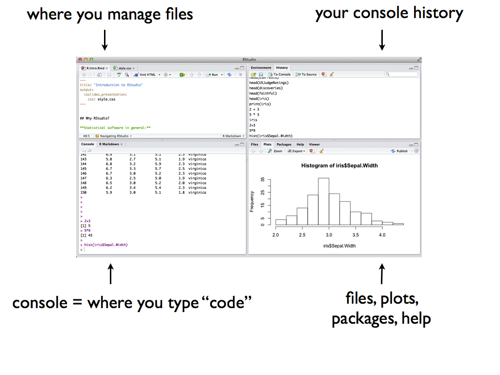
Figure 1.1: RStudio Interface

This short video tour of RStudio summarizes some basic features of the console.

Example 1.1 (Warm Up) Use RStudio as a simple calculator to do the following:

1. Perform a simple calculation: calculate 90/3.
2. RStudio has built-in functions to which we supply the necessary arguments: function(arguments). Use the built-in function sqrt to calculate the square root of 25.
3. Use the built-in function rep to repeat the number “5” eight times. (Type ?rep in the console and press Return. Check out the Help documentation for examples at the bottom.)
4. Use the seq function to create the vector (0, 3, 6, 9, 12). (Type ?seq in the console and press Return.)
5. Create a new vector by concatenating three repetitions of the vector from the previous part. (Type ?c in the console and press Return.)

Solution

90/3 
## [1] 30

sqrt(25)
## [1] 5

rep(5, times = 8)
## [1] 5 5 5 5 5 5 5 5

seq(0, 12, by = 3)
## [1]  0  3  6  9 12

rep(seq(0, 12, by = 3), times =  3)
##  [1]  0  3  6  9 12  0  3  6  9 12  0  3  6  9 12

rep(seq(0, 12, by = 3), each = 3) #notice the difference between the named input of times and each
##  [1]  0  0  0  3  3  3  6  6  6  9  9  9 12 12 12

Example 1.2 (Assignment) We often want to store our output for later use (why?). The basic idea in R:

`name <- output`

Copy and paste the following code into the console, line by line. NOTE: RStudio ignores any content after the #. Thus we use this to make ‘comments’ and organize our code.

#type square_3
square_3
    
#calculate 3 squared
3^2    
    
#store this as "square_3"
square_3 <- 3^2    
    
#type square_3 again!
square_3
    
#do some math with square_3
square_3 + 2

Data

Not only does “Data Science” require statistical software, it requires DATA! Consider the Google definition:

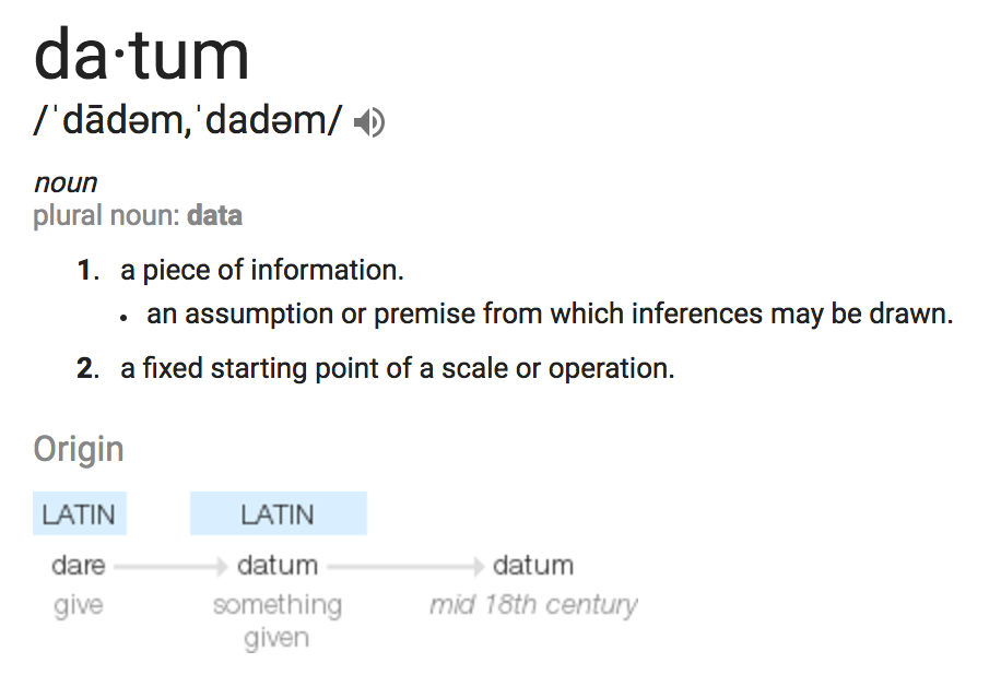
Figure 1.2: A datum.

With this definition in mind, which of the following are examples of data?

• tables

##   family father mother sex height nkids
## 1      1   78.5   67.0   M   73.2     4
## 2      1   78.5   67.0   F   69.2     4
## 3      1   78.5   67.0   F   69.0     4
## 4      1   78.5   67.0   F   69.0     4
## 5      2   75.5   66.5   M   73.5     4
## 6      2   75.5   66.5   M   72.5     4

• photo

• video

• text / tweets

We’ll mostly work with data that look like this:

##   family father mother sex height nkids
## 1      1   78.5   67.0   M   73.2     4
## 2      1   78.5   67.0   F   69.2     4
## 3      1   78.5   67.0   F   69.0     4
## 4      1   78.5   67.0   F   69.0     4
## 5      2   75.5   66.5   M   73.5     4
## 6      2   75.5   66.5   M   72.5     4

This isn’t as restrictive as it seems. We can convert the above signals: photos, videos, and text to a data table format!

Tidy Data

Example: After a scandal among FIFA officials, fivethirtyeight.com posted an analysis of FIFA viewership, “How to Break FIFA”. Here’s a snapshot of the data used in this article:

country	confederation	population_share	tv_audience_share	gdp_weighted_share
United States	CONCACAF	4.5	4.3	11.3
Japan	AFC	1.9	4.9	9.1
China	AFC	19.5	14.8	7.3
Germany	UEFA	1.2	2.9	6.3
Brazil	CONMEBOL	2.8	7.1	5.4
United Kingdom	UEFA	0.9	2.1	4.2
Italy	UEFA	0.9	2.1	4.0
France	UEFA	0.9	2.0	4.0
Russia	UEFA	2.1	3.1	3.5
Spain	UEFA	0.7	1.8	3.1

The data table above is in tidy format. Tidy data tables have three key features:

1. Each row represents a unit of observation (also referred to as a case).
   
2. Each column represents a variable (ie. an attribute of the cases that can vary from case to case). Each variable is one of two types:
   

• quantitative = numerical/numbers with units
  
• categorical = discrete possibilities/categories
  

3. Each entry contains a single data value; no analysis, summaries, footnotes, comments, etc., and only one value per cell

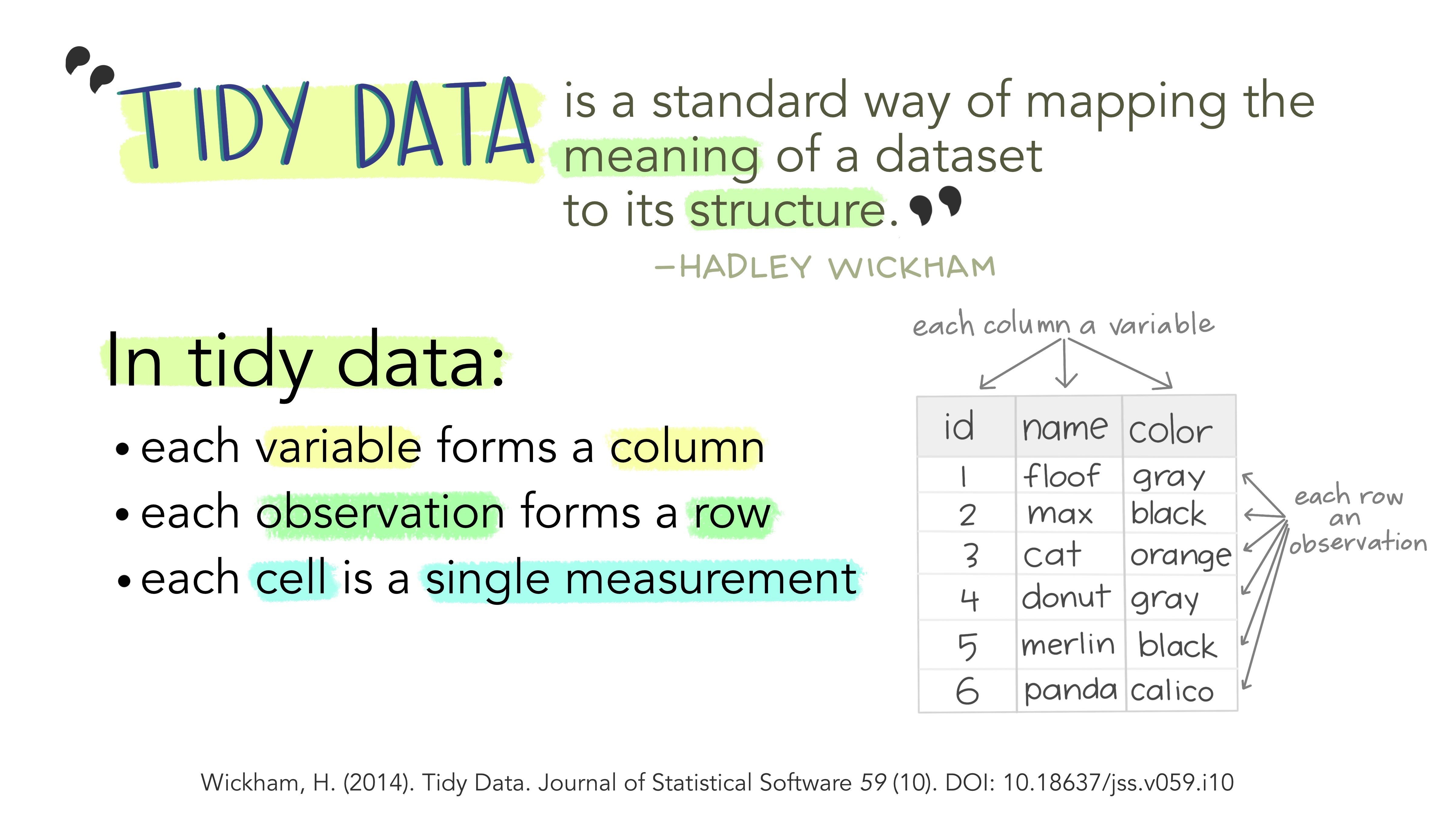
Tidy Data: Art by Allison Horst

Example 1.3 (Units of Observation and Variables) Consider the following in a group:

1. What are the units of observation in the FIFA data?
   
2. What are the variables? Which are quantitative? Which are categorical?
   
3. Are these tidy data?

Solution

1. A FIFA member country
2. country name, soccer or football confederation, country’s share of global population (percentage), country’s share of global world cup TV Audience (percentage), country’s GDP-weighted audience share (percentage)
3. Yes

Example 1.4 (Tidy vs. Untidy) Check out the following data. Explain to each other why they are untidy and how we can tidy them.

1. Data 1: FIFA

   country	confederation	population share	tv_share
   United States	CONCACAF	i don’t know*	4.3%	*look up later
   Japan	AFC	1.9	4.9%
   China	AFC	19.5	14.8%
   			total=24%

2. Data 2: Gapminder life expectancies by country

   	country	1952	1957	1962
   Asia	Afghanistan	28.8	30.3	32.0
   	Bahrain	50.9	53.8	56.9
   Africa	Algeria	43.0	45.7	48.3

Solution

1. There are notes such as “I don’t know” and “look up later” in columns with numeric values; the last row with the total is a summary. We could remove the text notes, replace it with the value if known, and remove the last row with the total summary.
2. The first column does not have a row name. It should be continent. Additionally, Bahrain needs a value for the continent.The column names ‘1952’, ‘1957’ and ‘1962’ are values not variables. The table should be ‘pivoted’ (more information on this coming soon!), so that there is an additional column named ‘year’ and each country has three observations (rows) associated with it (one for each year).

Data Basics in RStudio

For now, we’ll focus on tidy data. In a couple of weeks, you’ll learn how to “clean data” and turn untidy data into tidy data.

Example 1.5 (Importing Package Data) The first step to working with data in RStudio is getting it in there! How we do this depends on its format (eg: Excel spreadsheet, csv file, txt file) and storage locations (eg: online, within Wiki, desktop).

Luckily for us, the fifa_audience data are stored in the fivethirtyeight RStudio package. Copy and paste the following code into the Console and press Enter.

#download the data and information in the fivethirtyeight package (we only need to do this once)
install.packages('fivethirtyeight')

#load the fivethirtyeight package
library(fivethirtyeight)
    
#load the fifa data
data("fifa_audience")
    
#store this under a shorter, easier name
fifa <- fifa_audience

Example 1.6 (Examining Data Structures) Before we can analyze our data, we must understand its structure. Try out the following functions (copy and paste into the Console). For each, make a note that describes its action.

#(what does View do?)
View(fifa)  

#(what does head do?)
head(fifa)  

#(what does dim do?)
dim(fifa)           

#(what does names do?)
names(fifa)         

Solution

#View() opens up a new tab with a spreadsheet preview of the data to visually explore the data. It is commented out in the Rmarkdown file because this is an interactive feature
#View(fifa)  

#head() gives the first 6 (default number) rows of a data set
head(fifa)  
## # A tibble: 6 × 5
##   country        confederation population_s…¹ tv_au…² gdp_w…³
##   <chr>          <chr>                  <dbl>   <dbl>   <dbl>
## 1 United States  CONCACAF                 4.5     4.3    11.3
## 2 Japan          AFC                      1.9     4.9     9.1
## 3 China          AFC                     19.5    14.8     7.3
## 4 Germany        UEFA                     1.2     2.9     6.3
## 5 Brazil         CONMEBOL                 2.8     7.1     5.4
## 6 United Kingdom UEFA                     0.9     2.1     4.2
## # … with abbreviated variable names ¹​population_share,
## #   ²​tv_audience_share, ³​gdp_weighted_share

#dim() gives the number of rows and number of columns
dim(fifa)           
## [1] 191   5

#names() gives the names of the columns/variables
names(fifa)   
## [1] "country"            "confederation"     
## [3] "population_share"   "tv_audience_share" 
## [5] "gdp_weighted_share"

Example 1.7 (Codebooks) Data are also only useful if we know what they measure! The fifa data table is tidy; it doesn’t have any helpful notes in the data itself.

Rather, information about the data is stored in a separate codebook. Codebooks can be stored in many ways (eg: Google docs, word docs, etc). Here the authors have made their codebook available in RStudio (under the original fifa_audience name). Check it out (run the following code in the console):

?fifa_audience

1. What does population_share measure?
2. What are the units of population_share?

Solution

1. Country’s share of global population
2. Percentage between 0 and 100

Example 1.8 (Examining a Single Variable) Consider the following:

1. We might want to access and focus on a single variable. To this end, we can use the $ notation (see below). What are the values of tv_audience_share? Of confederation? Is it easy to figure out?

fifa$tv_audience_share
fifa$confederation

Solution

1. The values of tv_audience_share are numerical values between 0 and 7.1. By scanning through the long list, it looks like the values of confederation are words (a string of alphabetical characters): OFC, CAF, AFC, UEFA, CONCACAF, CONMEBOL.

It’s important to understand the format/class of each variable (quantitative, categorical, date, etc) in both its meaning and its structure within RStudio:

class(fifa$tv_audience_share)
class(fifa$confederation)

2. If a variable is categorical (in factor format), we can determine its levels / category labels. What are the value of confederation?

levels(fifa$confederation) #it is in character format
levels(factor(fifa$confederation)) #we can convert to factor format

Solution

2. The values of confederation are words, also known as strings of characters in computing languages (indicated by the quotes around them): “AFC”, “CAF”, “CONCACAF”, “CONMEBOL”, “OFC”, “UEFA”.

R Markdown and Reproducible Research

Reproducible research is the idea that data analyses, and more generally, scientific claims, are published with their data and software code so that others may verify the findings and build upon them. - Reproducible Research, Coursera

Useful Resources:

1. R Markdown Quick Tour
   
2. R Markdown Cheatsheet
3. R Markdown Reference Guide

Research often makes claims that are difficult to verify. A recent study of published psychology articles found that less than half of published claims could be reproduced. One of the most common reasons claims cannot be reproduced is confusion about data analysis. It may be unclear exactly how data was prepared and analyzed, or there may be a mistake in the analysis.

In this course we will use an innovative format called R Markdown that dramatically increases the transparency of data analysis. R Markdown interleaves data, R code, graphs, tables, and text, packaging them into an easily publishable format.

To use R Markdown, you will write an R Markdown formatted file in RStudio and then ask RStudio to knit it into an HTML document (or occasionally a PDF or MS Word document).

Example 1.9 (Deduce the R Markdown Format) Look at this Sample RMarkdown and the HTML webpage it creates. Consider the following and discuss:

1. How are bullets, italics, and section headers represented in the R Markdown file?
2. How does R code appear in the R Markdown file?
3. In the HTML webpage, do you see the R code, the output of the R code, or both?

Solution

Bullets are represented with * and +
Italics are represented with * before and after a word or phrase
Section headers are represented with #

R code chunks are between 3 tick marks at the beginning and end; it is R code if there is an r in curly braces
  
If echo=FALSE in curly braces, the code is not shown. Otherwise, both code and output are shown by default.

 

Now take a look at the R Markdown cheatsheet. Look up the R Markdown features from the previous question on the cheatsheet. There’s a great deal more information there.

Practice

Complete the following. If you get stuck along the way, refer to the R Markdown cheatsheet linked above, search the web for answers, and/or ask for help!

Exercise 1.1 (Your First R Markdown File) Create a new R Markdown about your favorite food.

1. Create a new file in RStudio (File -> New File -> R Markdown) with a Title of First_Markdown. Save it to a new folder on your Desktop called COMP_STAT_112; within that new folder, create another new folder called Assignment_01.
   
2. Make sure you can compile/render (Knit) the Markdown into a webpage (html file).
   
3. Add a new line between title and output that reads: author: Your Name.
4. Delete everything from ## RMarkdown and below. Create a new section by typing ## Favorite Food.
5. Create a very brief essay about your favorite food. Make sure to include:
   

• A picture from the web
  
• A bullet list
  
• A numbered list
  

6. Compile (Knit) the document into an html file and make sure it looks like you want it to.

Exercise 1.2 (New Data!) There’s a data set named comic_characters in the fivethirtyeightdata package.

Install the package by running the following in the console:

install.packages('fivethirtyeightdata', repos = 'https://fivethirtyeightdata.github.io/drat/', type = 'source')

Check out the codebook (hint: use ?) to understand what these data measure.

Add a second section to your RMarkdown file that you’ve created (with ##), and then use code chunks and R commands to perform/answer the following tasks/questions:

1. Load the comic_characters data.
   
2. What are the units of observation? How many observations are there?
   
3. In a new code chunk, print out the first 12 rows of the data set.
4. Get a list of all variable names.
   
5. What’s the class of the date variable?
   
6. List all of the unique entries in the gsm variable (no need to include NA).
7. Compile the document into an html file.

Appendix: R Functions

R as a calculator

Function/Operator	Action	Example
/	Division	90/30
*	Multiplication	2*5
+	Addition	1+1
-	Subtraction	1-1
^	Exponent/Power to	3^2
sqrt(x)	Square root	sqrt(25)

R Basics

Function/Operator	Action	Example
install.packages('packagename')	Download a R package (function, data, etc.) from repository	install.packages('fivethirtyeight')
library(packagename)	Access a downloaded R package	library(fivethirtyeight)
?function_object_name	Opens the help/documentation for the function or object	?seq
rep(x, times, each)	Repeat x a # times	rep(5,8)
seq(from, to, by)	Sequence generation	seq(0, 12, by = 2)
name <- value_output	Assign value or output to a name	squared_3 <- 3^2
View(x)	Open spreadsheet viewer of dataset	View(fifa_audience)
head(x)	Print the first 6 rows of a dataset	head(fifa_audience)
dim(x)	Print the dimensions (number of rows and columns) of a dataset	dim(fifa_audience)
names(x)	Print the names of the variables in a dataset	names(fifa_audience)
$	Used to access one variable in a data set based on its name	fifa_audience$confederation
class(x)	Print the class types argument or input	class(fifa_audience$confederation)
factor(x)	Converts the argument or input to a factor class type (categorical variable)	factor(fifa_audience$confederation)
levels(x)	Prints the unique categories of a factor	levels(factor(fifa_audience$confederation))