1.1 Data Types

In this class, we focus on temporal data, in which we have repeated measurements over time on the same units, and spatial data, in which the measurement location plays a meaningful role in the analysis.

There are two types of temporal data we discuss in this class.

1. We call temporal data a time series if we have measurements on a smaller number of units or subjects taken at many (typically \(>20\)) regular and equally-spaced times.

2. We call temporal data longitudinal data if we have measurements on many units or subjects taken at approximately 2 to 20 observations times (potentially irregular, unequally-spaced times) that may differ between subjects. If we have repeated measurements on each subject in different conditions rather than necessarily over some time, we call this data repeated measures data, but the methods will be the same for both longitudinal and repeated measures data.

Spatial data can be measured as

1. observations at a point in space, typically measured using a longitude and latitude coordinate system, or

2. areal units, which are aggregated summaries based on natural or societal boundaries such as county districts, census tracts, postal code areas, or any other arbitrary spatial partition.

The common thread between these types of data is that observations measured closer in time or space tend to be more similar (more positively correlated) than observations measured further away in time or space.

1.1.1 Data Type Examples

Here are some examples of these types of data.

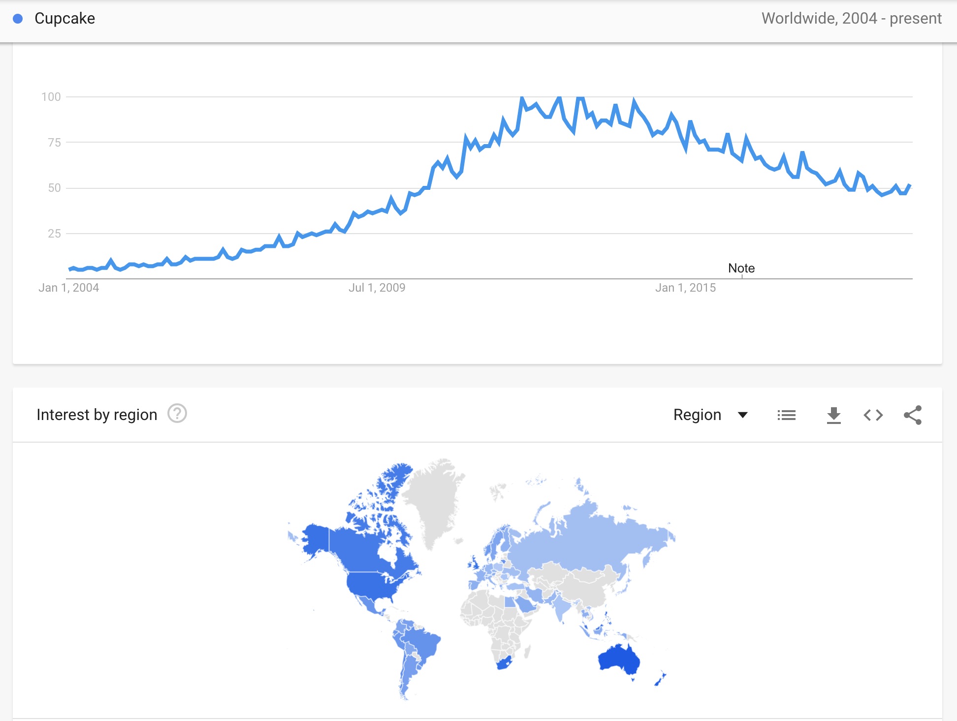
• Time series: Below are the daily use frequency for the search term “cupcake” from Google Trends (source: https://trends.google.com/trends/explore?q=%2Fm%2F03p1r4&date=all). While there is a spatial component (areal units are countries), we could focus solely on the time series and ignore the country. We notice a larger overall trend of increase and then a slight decrease in the search frequency. We also note there may be a cyclic pattern that may indicate that there are predictable times of the year in which searches for “cupcake” might be more or less popular.

• Longitudinal Data: Below are measurements of reasoning ability over time on a group of subjects from the ACTIVE clinical trial. In the plot, each individual is represented by one connected line segment or trajectory (source: https://www.icpsr.umich.edu/icpsrweb/ICPSR/studies/4248?q=Advanced+Cognitive+Training+for+Independent+and+Vital+Elderly+%2528ACTIVE%2529). We see that among the subjects that were randomized to the Reasoning Training group, on average their reasoning measure increased after training and then leveled off similar to other groups. We also see quite a bit of variation in reasoning abilities between subjects and across time within a subject.

source('Cleaning.R')

activeLong %>%
  ggplot(aes(x = Years, y = Reasoning)) +
  geom_point() + 
  geom_line(aes(group = factor(AID))) + 
  geom_smooth(method = 'loess',color = 'blue' , se = FALSE) +
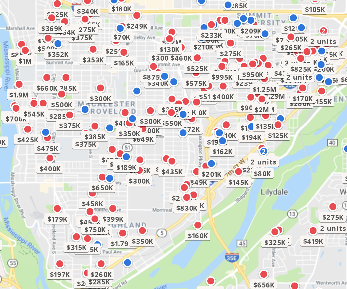
  facet_wrap(~ INTGRP)

• Spatial Point Referenced Data: Below are homes for sale in St. Paul and are spread out in space (longitude, latitude) (source: https://www.zillow.com/homes/for_sale/pmf,pf_pt/globalrelevanceex_sort/44.974332,-93.09617,44.886708,-93.219767_rect/12_zm/). We might be able to explain why some houses cost more than others using building characteristics (number of bedrooms, bathrooms, etc.). Even after accounting for those differences, houses close together have similar values due to other intangible factors about the location. We’ll need to account for this dependency in models to predict home prices.