7.1 Mapping in R
The technology available in R is rapidly evolving and improving. In this set of notes, I’ve highlighted some basics for working with spatial data in R but I’m listing some good resources below.
- https://cran.r-project.org/web/views/Spatial.html (last updated in 2022)
- https://r-spatial.github.io/sf/index.html (last updated in 2022)
- https://geocompr.robinlovelace.net/intro.html (last updated in 2022)
- https://cengel.github.io/R-spatial/ (last updated in 2019)
- http://www.nickeubank.com/gis-in-r/
7.1.1 Coordinate Reference Systems (CRS)
CRS provides a standardized way of describing locations. There are two main packages in R that are used to assign and transform CRS in R, sf and rgdal.
In general, there are three main attributes of CRS: projection, datum, and ellipsoid.
7.1.1.1 Ellipsoid & Datum
The ellipse describes the generalized shape of the earth (The earth is generally a sphere but with some bulges at the equator). The common ellipse are WGS84 and GRS80 but there are more regional ellipsoids that are more accurate for specific regions. The datum defines the origin and orientation of the coordinate axes. Together these form a globe, which is a 3D ellipse with longitudinal and latitude coordinates.
The 3 most common datum/ellipse used in U.S.:
WGS84 (EPSG: 4326)
+init=epsg:4326 +proj=longlat +ellps=WGS84
+datum=WGS84 +no_defs +towgs84=0,0,0
## CRS used by Google Earth and the U.S. Department of Defense for all their mapping.
## Tends to be used for global reference systems.
## GPS satellites broadcast the predicted WGS84 orbits.
NAD83 (EPSG: 4269)
+init=epsg:4269 +proj=longlat +ellps=GRS80 +datum=NAD83
+no_defs +towgs84=0,0,0
##Most commonly used by U.S. federal agencies.
## Aligned with WGS84 at creation, but has since drifted.
## Although WGS84 and NAD83 are not equivalent, for most applications they are very similar.
NAD27 (EPSG: 4267)
+init=epsg:4267 +proj=longlat +ellps=clrk66 +datum=NAD27
+no_defs
+nadgrids=@conus,@alaska,@ntv2_0.gsb,@ntv1_can.dat
## Has been replaced by NAD83, but is still encountered!
For more resources related to EPSG, go to https://epsg.io/ and https://spatialreference.org/.
7.1.1.2 Projection
Lastly, we must project the 3D ellipse on a 2D surface to make a map with Easting and Northing coordinates. It is impossible to flatten a round object without distortion, and this results in trade-offs between area, direction, shape, and distance. For example, there is a trade-off between distance and direction because both features can not be simultaneously preserved. There is no “best” projection, but some projections are better suited to different applications.
Check out more info about projections: https://www.arcgis.com/apps/MapJournal/index.html?appid=31484c80dba54a058369dfb8e9ced549
In general, I’ll provide code for you, but it is important to think about what format your location has been recorded in.
7.1.2 R Packages
The following R packages support spatial data classes (data sets that are indexed with geometries):
sf: genericmaps: polygon maps
The following R packages support geostatistical/point-referenced data:
gstat: classical geostatisticsgeoR: model-based geostatisticsRandomFields: stochastic processesakima: interpolation
The following R packages support regional/areal data:
spdep: spatial dependencespgwr: geographically weighted regression
The following R packages support point patterns/processes data:
spatstat: parametric modeling, diagnosticssplancs: nonparametric, space-time
7.1.3 Visualizations
In general, if you have geometries (points, polygons, lines, etc) that you want to plot, you can use geom_sf() with ggplot(). See https://ggplot2.tidyverse.org/reference/ggsf.html for more details.
7.1.3.1 Plotting points
If you have x and y coordinates (longitude and latitude over a small region), we can use our typically plotting tools in ggplot2 package using the x and y coordinates as the values of x and y in geom_point(). Then you can color the points according to a covariate or outcome variable.
If you have longitude and latitude over the globe or a larger region, then you’ll need to project those coordinates onto a 2D surface. You can do this using the sf package and st_transform() after specifying the CRS (documentation: https://www.rdocumentation.org/packages/sf/versions/0.8-0/topics/st_transform).
library(maps)

# Points without CRS
us.cities %>%
  ggplot(aes(x = long, y = lat, color = log(pop))) +
  geom_point() + theme_classic()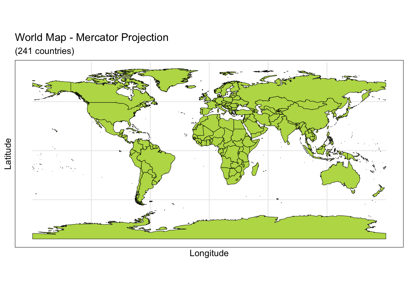
# Points with a CRS
states <- st_as_sf(maps::map("state", plot = FALSE, fill = TRUE))

us.cities %>%
  st_as_sf(coords = c('long','lat'),crs = st_crs(states)$proj4string) %>% head()
## Simple feature collection with 6 features and 4 fields
## Geometry type: POINT
## Dimension: XY
## Bounding box: xmin: -123.1 ymin: 31.58 xmax: -73.8 ymax: 44.62
## Geodetic CRS: +proj=longlat +ellps=clrk66 +no_defs
## name country.etc pop capital geometry
## 1 Abilene TX TX 113888 0 POINT (-99.74 32.45)
## 2 Akron OH OH 206634 0 POINT (-81.52 41.08)
## 3 Alameda CA CA 70069 0 POINT (-122.3 37.77)
## 4 Albany GA GA 75510 0 POINT (-84.18 31.58)
## 5 Albany NY NY 93576 2 POINT (-73.8 42.67)
## 6 Albany OR OR 45535 0 POINT (-123.1 44.62)us.cities %>%
st_as_sf(coords = c('long','lat'),crs = st_crs(states)$proj4string) %>%
ggplot() +
geom_sf(aes(color = log(pop))) +
geom_sf(data=states, alpha = 0.1) + theme_classic()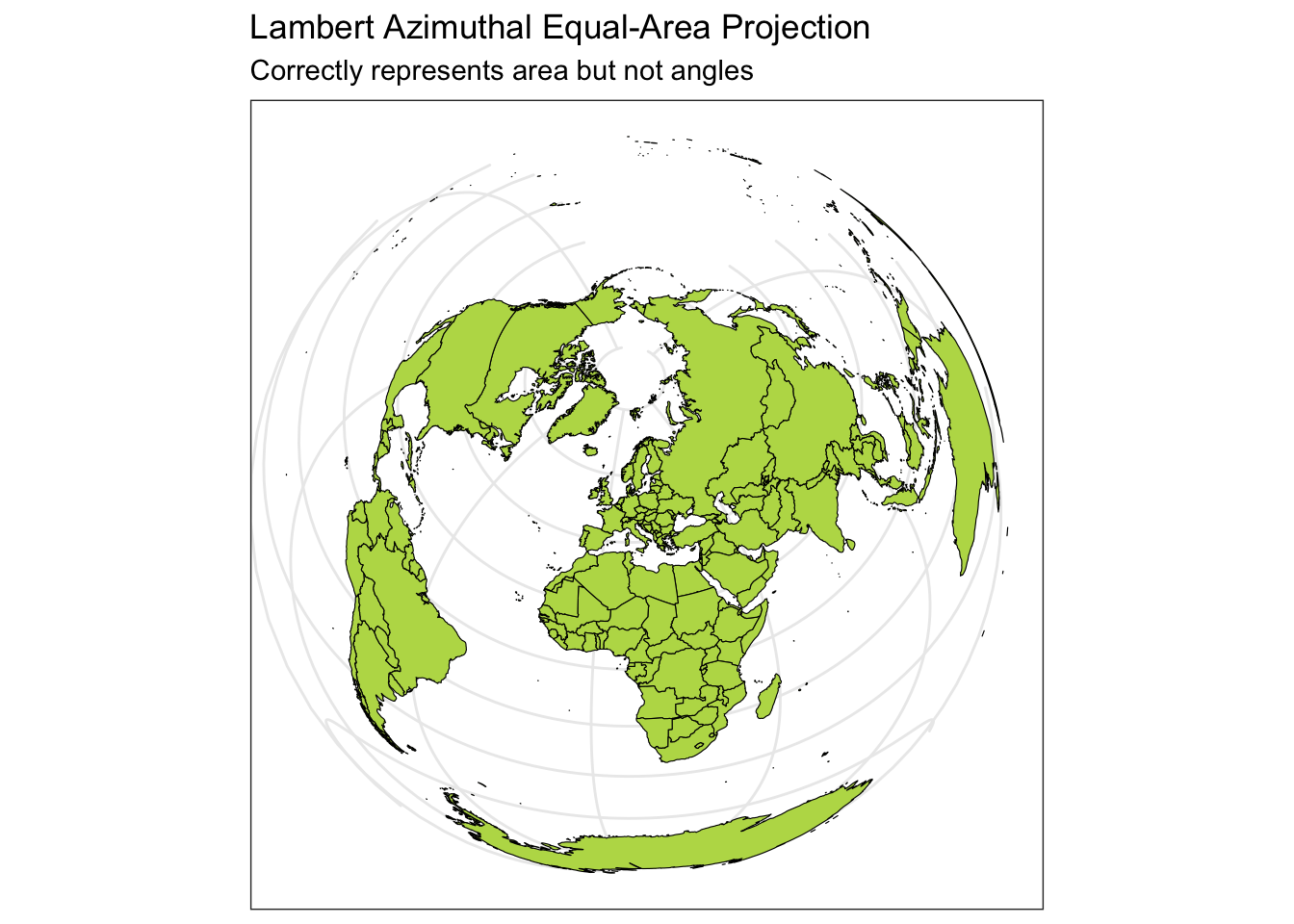
# Mercator Projection
us.cities %>%
  st_as_sf(coords = c('long','lat'), crs = st_crs(states)$proj4string) %>%
  sf::st_transform(crs = "+proj=tmerc") %>%
  ggplot() +
  geom_sf(aes(color = log(pop))) +
  geom_sf(data=states %>% sf::st_transform(crs = "+proj=tmerc"), alpha = 0.1) + theme_classic()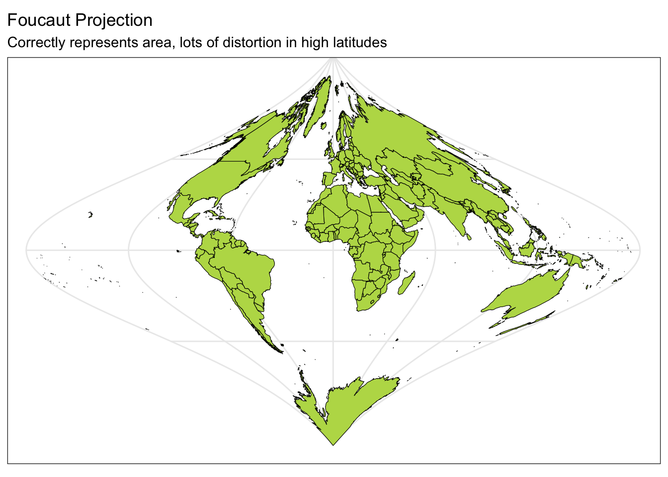
# Subset to Contiguous US States
us.cities %>%
  filter(!(country.etc %in% c('HI','AK'))) %>%
  st_as_sf(coords = c('long','lat'), crs = st_crs(states)$proj4string) %>%
  ggplot() +
  geom_sf(aes(color = log(pop))) +
  geom_sf(data=states, alpha = 0.1) + theme_classic()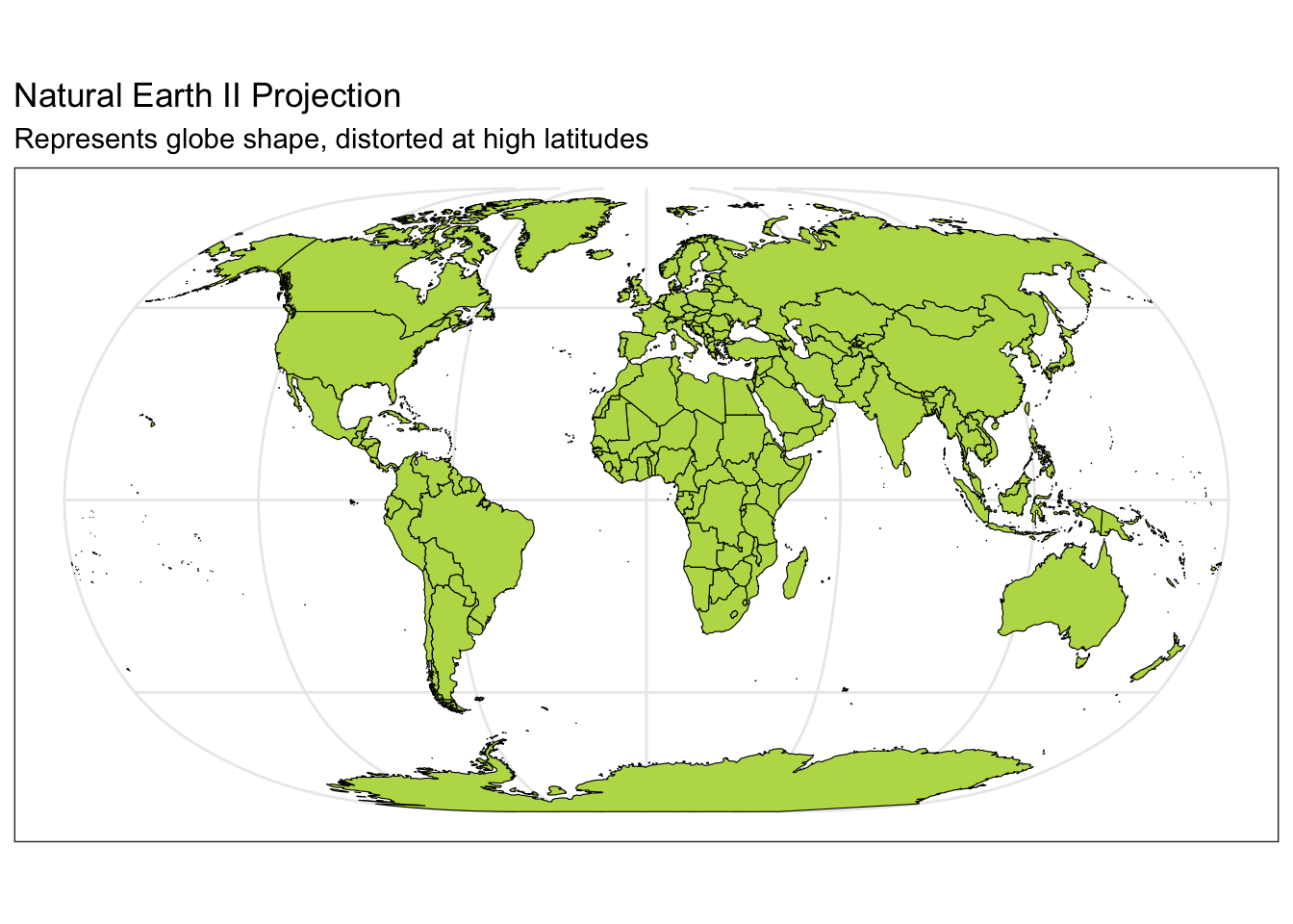
# Subset to MN
us.cities %>%
  filter((country.etc == 'MN')) %>%
  st_as_sf(coords = c('long','lat'), crs = st_crs(states)$proj4string) %>%
  ggplot() +
  geom_sf(aes(color = log(pop))) +
  geom_sf(data=states %>% filter(ID == 'minnesota'), alpha = 0.1) + theme_classic()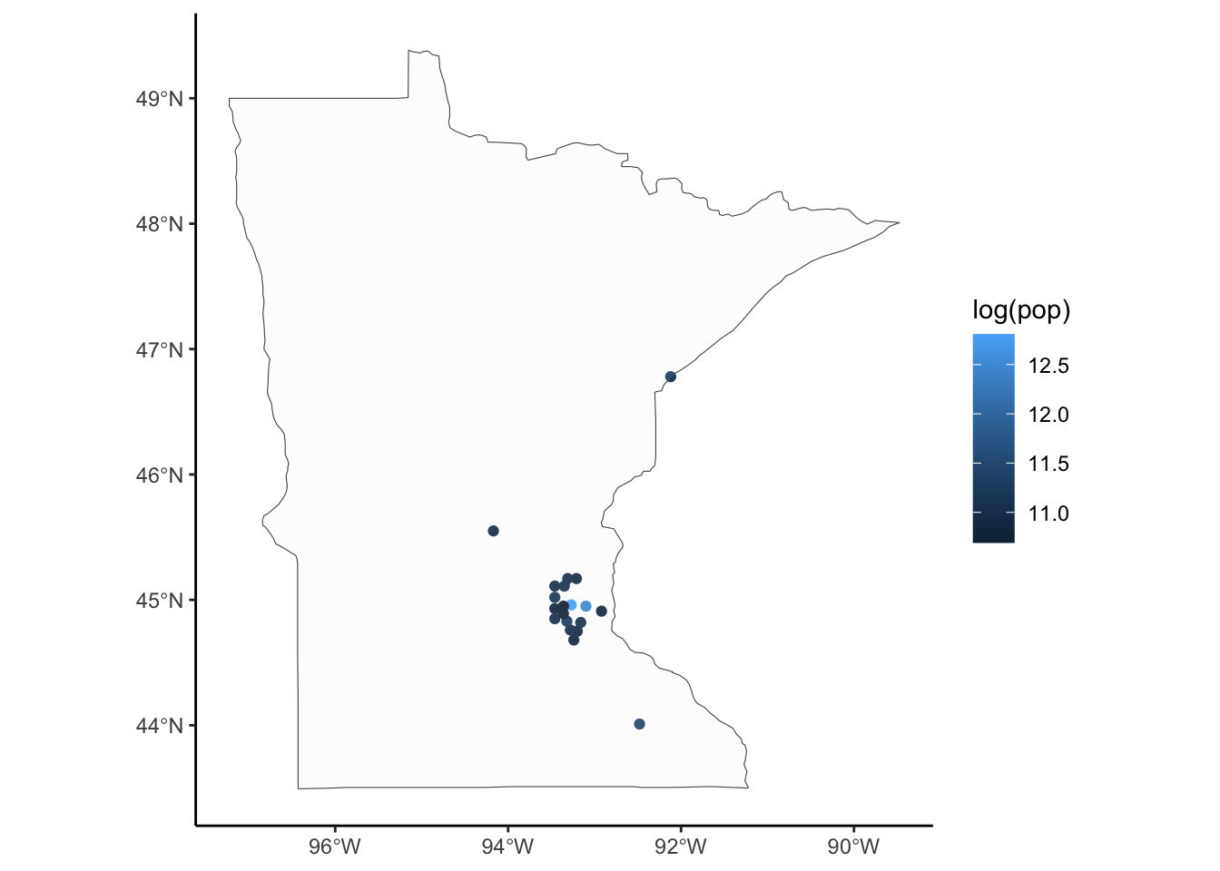
7.1.3.2 Plotting polygons
If you have areal data, then you’ll need shapefiles that provide boundaries for those polygons. These are often provided by city, state, or federal governments. We can read them into R with st_read() in the sf package. Once we have that stored object, we can view shapefile metadata using the st_geometry_type(), st_crs() and st_bbox(). These tell you about the type of geometry stored about the shapes, the CRS, and the bounding box that determines the study area of interest.
If we have data that are originally as points that we will aggregate to a polygon level, then we could use code such as the one below to join together the summaries at an average longitude and latitude coordinate with the shapefiles by whether the longitude and latitude intersect with the polygon.
#join the shapefile and our data summaries with a common polygon ID variable
fulldat <- left_join(shapefile, dat)
If we have data that are originally as points that we will aggregate to a polygon level, then we could use code such as the one below to join together the summaries at an average longitude and latitude coordinate with the shapefiles by whether the longitude and latitude intersect with the polygon.
# make our data frame a spatial data frame
dat <- st_as_sf(originaldatsum, coords = c('Longitude','Latitude'))
#copy the coordinate reference info from the shapefile onto our new data frame
st_crs(dat) <- st_crs(shapefile)

#join the shapefile and our data summaries
fulldat <- st_join(shapefile, dat, join = st_intersects)
If you are working with U.S. counties or states, or global countries, then the shapefiles are already available in the map package. You’ll need to use the ID variable to join this data with your polygon-level data.
## Simple feature collection with 6 features and 1 field
## Geometry type: MULTIPOLYGON
## Dimension:     XY
## Bounding box:  xmin: -124.4 ymin: 30.24 xmax: -71.78 ymax: 42.05
## Geodetic CRS:  +proj=longlat +ellps=clrk66 +no_defs +type=crs
##                      ID                           geom
## alabama         alabama MULTIPOLYGON (((-87.46 30.3...
## arizona         arizona MULTIPOLYGON (((-114.6 35.0...
## arkansas       arkansas MULTIPOLYGON (((-94.05 33.0...
## california   california MULTIPOLYGON (((-120 42.01,...
## colorado       colorado MULTIPOLYGON (((-102.1 40.0...
## connecticut connecticut MULTIPOLYGON (((-73.5 42.05...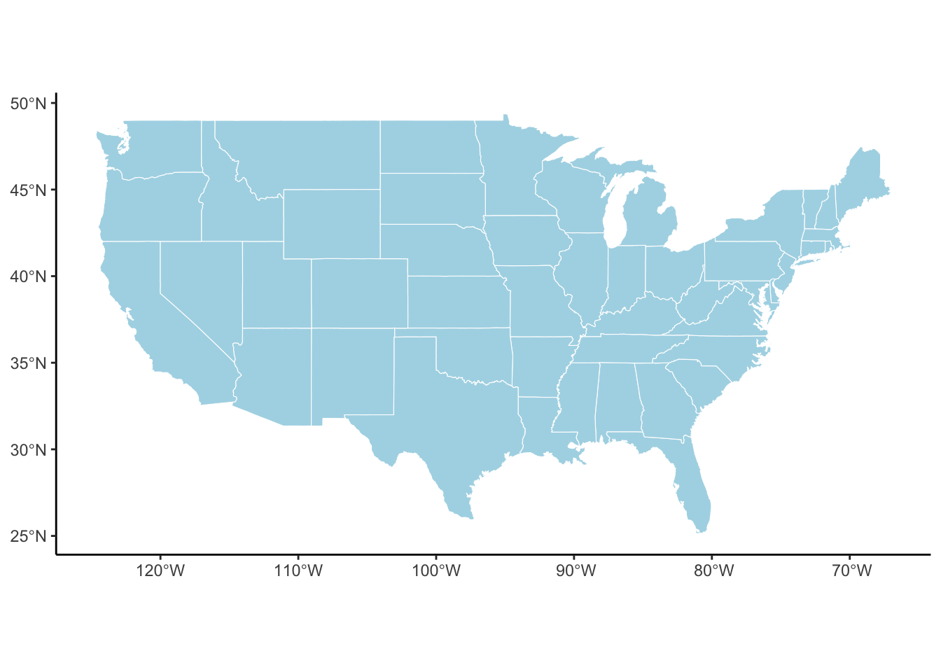
## Simple feature collection with 6 features and 1 field
## Geometry type: MULTIPOLYGON
## Dimension:     XY
## Bounding box:  xmin: -88.02 ymin: 30.24 xmax: -85.06 ymax: 34.27
## Geodetic CRS:  +proj=longlat +ellps=clrk66 +no_defs +type=crs
##                              ID                           geom
## alabama,autauga alabama,autauga MULTIPOLYGON (((-86.51 32.3...
## alabama,baldwin alabama,baldwin MULTIPOLYGON (((-87.94 31.1...
## alabama,barbour alabama,barbour MULTIPOLYGON (((-85.43 31.6...
## alabama,bibb       alabama,bibb MULTIPOLYGON (((-87.02 32.8...
## alabama,blount   alabama,blount MULTIPOLYGON (((-86.96 33.8...
## alabama,bullock alabama,bullock MULTIPOLYGON (((-85.67 31.8...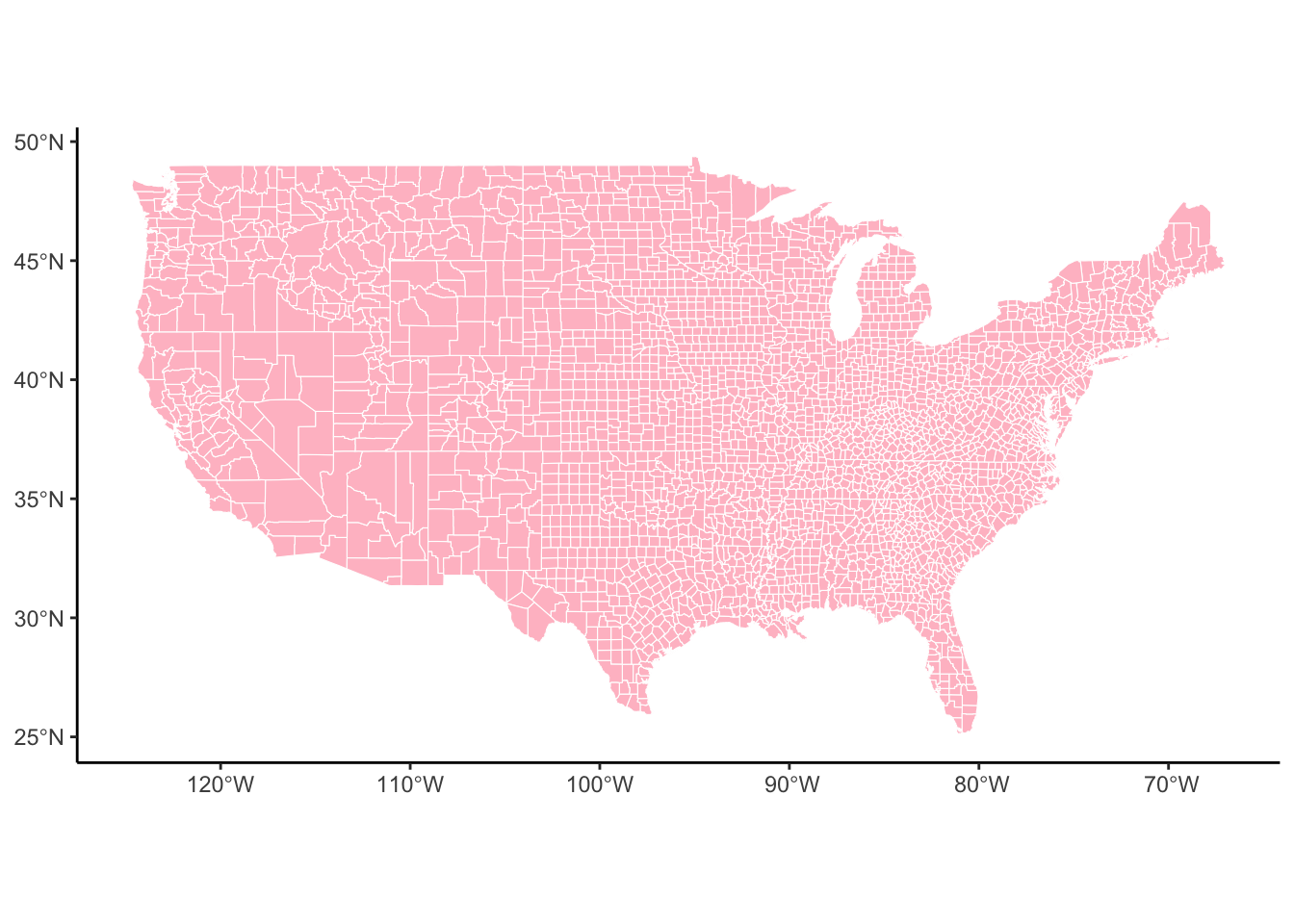
## Simple feature collection with 6 features and 1 field
## Geometry type: MULTIPOLYGON
## Dimension:     XY
## Bounding box:  xmin: -70.07 ymin: -18.02 xmax: 74.89 ymax: 70.06
## Geodetic CRS:  +proj=longlat +ellps=clrk66 +no_defs +type=crs
##                      ID                           geom
## Aruba             Aruba MULTIPOLYGON (((-69.9 12.45...
## Afghanistan Afghanistan MULTIPOLYGON (((74.89 37.23...
## Angola           Angola MULTIPOLYGON (((23.97 -10.8...
## Anguilla       Anguilla MULTIPOLYGON (((-63 18.22, ...
## Albania         Albania MULTIPOLYGON (((20.06 42.55...
## Finland         Finland MULTIPOLYGON (((20.61 60.04...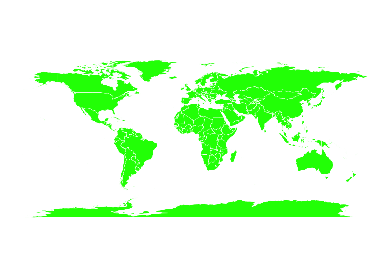
## [1] "+proj=longlat +ellps=clrk66 +no_defs"countries %>%
sf::st_transform(crs = "+proj=moll") %>%
ggplot() + geom_sf(color = 'white', fill = 'grey',size = 0.1) + theme_classic()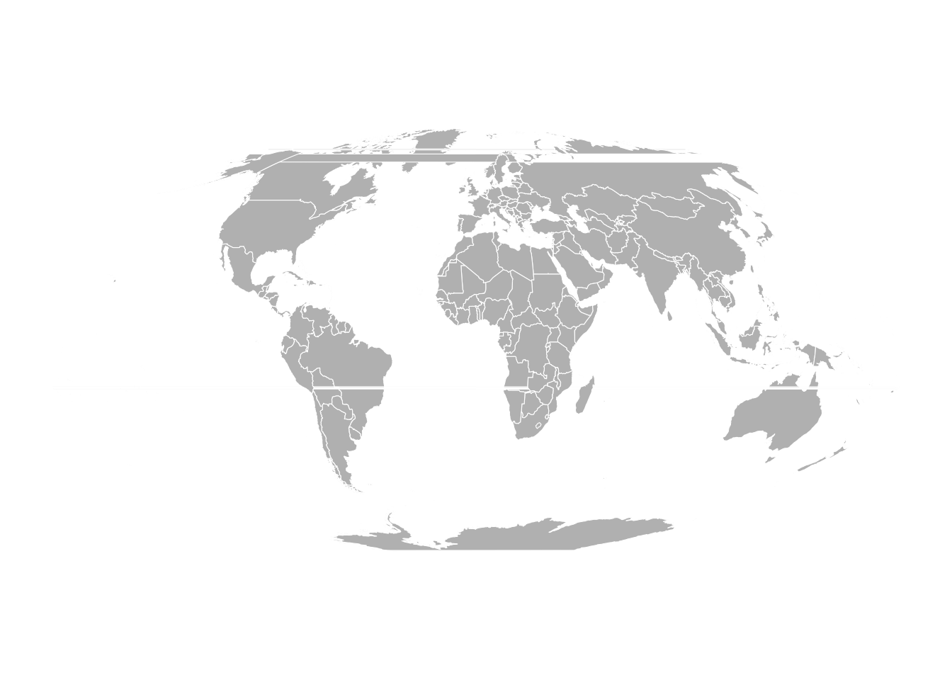
countries %>%
    sf::st_transform(crs = "+proj=tmerc") %>%
    ggplot() + geom_sf(color = 'white', fill = 'lightgrey',size = 0.1) + theme_classic()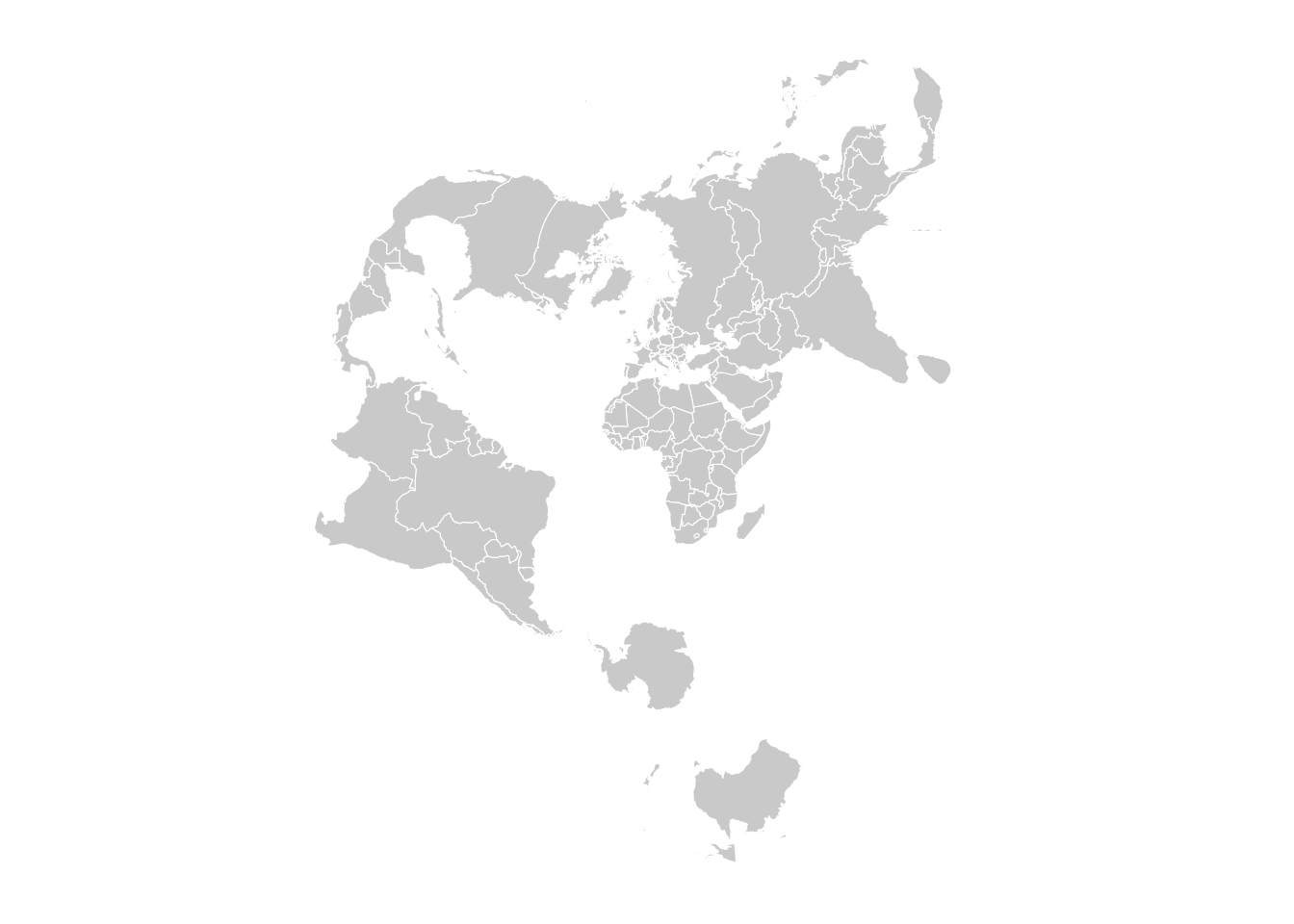
countries %>%
    sf::st_transform(crs = "+proj=laea +x_0=0 +y_0=0 +lon_0=-74 +lat_0=40") %>%
    ggplot() + geom_sf(color = 'white', fill = 'lightblue',size = 0.1) + theme_classic()
Once we have an sf object with attributes (variables) and geometry (polygons), we can use geom_sf(aes(fill = attribute)) to plot and color the polygons in the ggplot2 context with respect to an outcome variable.
#devtools::install_github("UrbanInstitute/urbnmapr")
library(urbnmapr) # projection with Alaska and Hawaii close to lower 48 states
get_urbn_map(map = "counties", sf = TRUE) %>%
    left_join(countydata) %>%
    ggplot() + geom_sf(aes(fill = horate), color = 'white',linewidth = 0.01) +
    labs(fill = 'Homeownership Rate') +
    scale_fill_gradient(high='white',low = 'darkblue',limits=c(0.25,0.85)) +
    theme_void()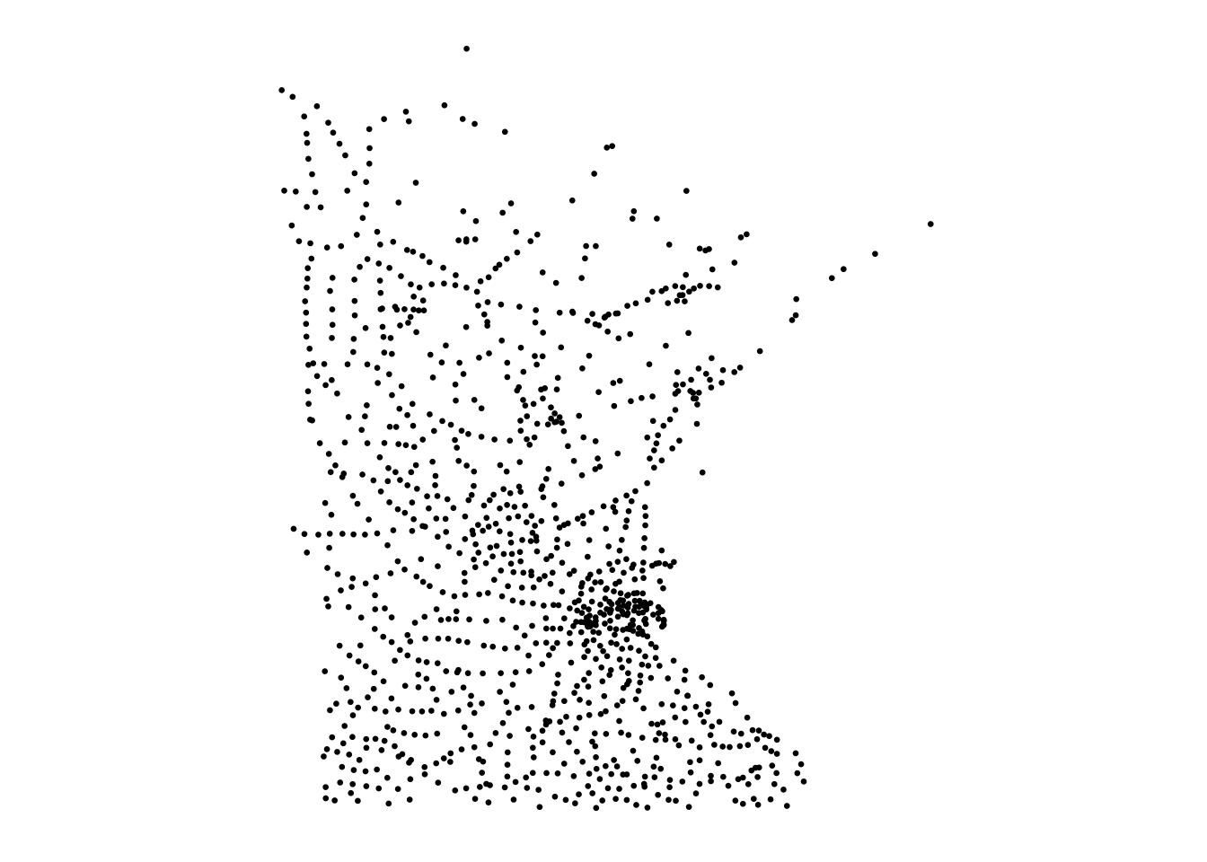
# Subset to MN
get_urbn_map(map = "counties", sf = TRUE) %>%
    left_join(countydata) %>%
    filter(stringr::str_detect(state_abbv,'MN')) %>%
    ggplot() + geom_sf(aes(fill = horate), color = 'white',linewidth = 0.05) +
    labs(fill = 'Homeownership Rate') +
  scale_fill_gradient(high='white',low = 'darkblue',limits=c(0.25,0.85)) +
  theme_void()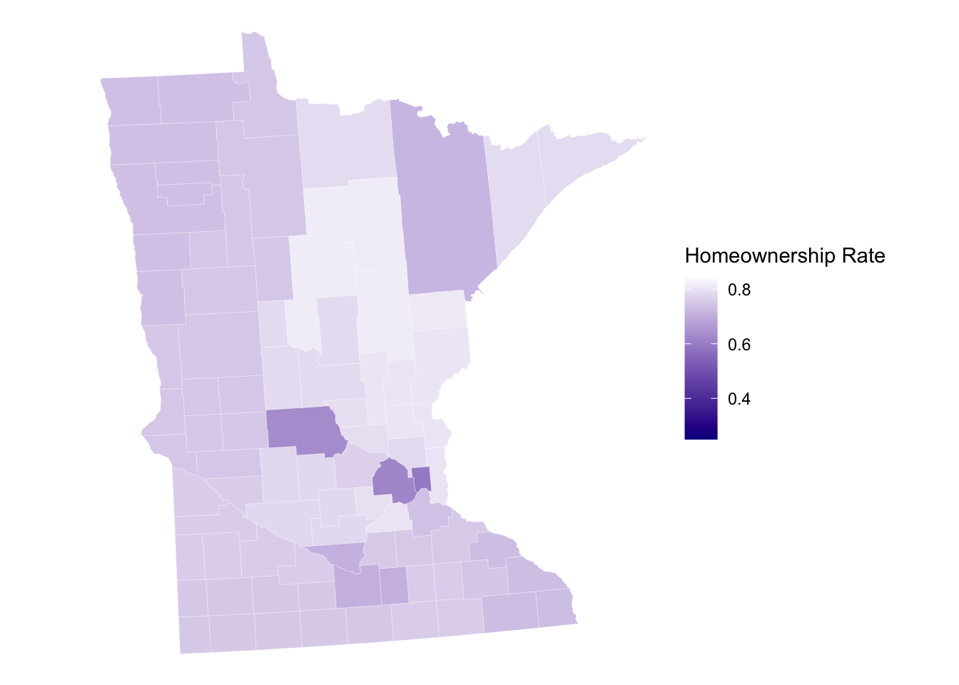
7.1.3.3 Google Map Background
Due to changes with the Google Maps API, a bit more work is needed to display a Google map as the background to your ggplot(). Here is a recent tutorial: https://www.littlemissdata.com/blog/maps. Since technology is always changing, this link may come outdated.
7.1.4 More R Resources
- sf package: https://r-spatial.github.io/sf/
- sf Cheat sheet: https://github.com/rstudio/cheatsheets/blob/main/sf.pdf
- Spatial Data Science: https://keen-swartz-3146c4.netlify.app/
- Geocomputation with R: https://geocompr.robinlovelace.net/index.html