8 Wrangling verbs

SETTLING IN

Try sitting next to someone you don’t know well. Introduce yourself!

Favorite fall activity?

Help each other with the following:

Prepare to take notes. Open the activity qmd file.

Learning goals

Explore the following wrangling verbs: select, mutate, filter, arrange, summarize, group_by

Additional resources

Watch:

Intro to dplyr (Lisa Lendway)
Demonstration of dplyr (Lisa Lendway)

Read:

Data Transformation (Wickham, Çetinkaya-Rundel, & Grolemund)
A Grammar for Data Wrangling (Baumer, Kaplan, and Horton)

8.1 Data wrangling motivation

Recall the elections data by U.S. county:

# Load tidyverse & data
library(tidyverse)
elections <- read.csv("https://mac-stat.github.io/data/election_2020_county.csv")

We’ve used data viz to explore some general patterns in the election outcomes. For example, a map!

# Get a background map
library(socviz)
data(county_map)

# Make a choropleth map
library(RColorBrewer)  # For the color scale
library(ggthemes) # For theme_map
elections %>% 
  mutate(county_fips = as.character(county_fips)) %>% 
  mutate(county_fips = 
           ifelse(nchar(county_fips) == 4, paste0("0", county_fips), county_fips)) %>% 
  ggplot(aes(map_id = county_fips, fill = cut(repub_pct_20, breaks = seq(0, 100, by = 10)))) +
    geom_map(map = county_map) +
    scale_fill_manual(values = rev(brewer.pal(10, "RdBu")), name = "% Republican") +
    expand_limits(x = county_map$long, y = county_map$lat)  + 
    theme_map() +
    theme(legend.position = "right") + 
    coord_equal()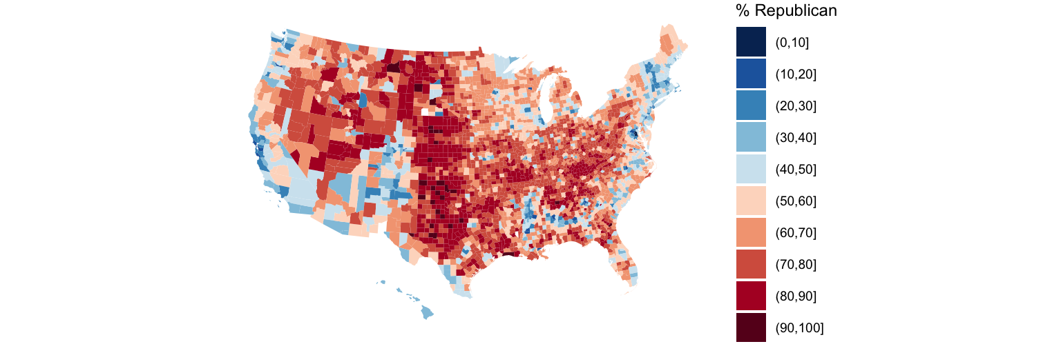

Consider some fairly basic follow-up questions, each of which we cannot answer precisely (or sometimes even at all) using our data viz tools:

How many total people voted for the Democratic and Republican candidates in 2020?
What about in each state?
In just the state of Minnesota:
- Which counties had the highest and lowest Democratic vote in 2020?
- How did the Democratic vote in each county change from 2016 to 2020?

GOALS OF UNIT 2: DATA WRANGLING

We really cannot do anything with data (viz, modeling, etc) unless we can wrangle the data. The following is a typical quote. I agree with the 90% – data wrangling isn’t something we have to do before we can do data science, it is data science! But let’s rethink the 10% – data wrangling is a fun and empowering puzzle!

The goals of Unit 2 are to explore how to:

Get data into the tidy shape / format we need for analysis. For example, we might want to:
- keep only certain observations
- define new variables
- reformat or “clean” existing variables
- combine various datasets
- process “string” or text data
Numerically (not just visually) explore and summarize various characteristics of the variables in our dataset.

TIDYVERSE WRANGLING TOOLS

We’ll continue to use packages that are part of the tidyverse, which share a common general grammar and structure.

8.2 Warm-up

There are lots and lots of steps that can go into data wrangling, thus lots and lots of relevant R functions. BUT just 6 functions can get us very far. People refer to these as the 6 main wrangling verbs or functions:

why “verbs”? in the tidyverse grammar, functions serve as action words
the 6 verbs are all stored in the dplyr package within the tidyverse
each verb acts on a data frame and returns a data frame

verb	action
`arrange`	arrange the rows according to some column
`filter`	filter out or obtain a subset of the rows
`select`	select a subset of columns
`mutate`	mutate or create a column
`summarize`	calculate a numerical summary of a column
`group_by`	group the rows by a specified column

EXAMPLE 1

head(elections)
##   state_name state_abbr historical    county_name county_fips total_votes_20
## 1    Alabama         AL        red Autauga County        1001          27770
## 2    Alabama         AL        red Baldwin County        1003         109679
## 3    Alabama         AL        red Barbour County        1005          10518
## 4    Alabama         AL        red    Bibb County        1007           9595
## 5    Alabama         AL        red  Blount County        1009          27588
## 6    Alabama         AL        red Bullock County        1011           4613
##   repub_pct_20 dem_pct_20 winner_20 total_votes_16 repub_pct_16 dem_pct_16
## 1        71.44      27.02     repub          24661        73.44      23.96
## 2        76.17      22.41     repub          94090        77.35      19.57
## 3        53.45      45.79     repub          10390        52.27      46.66
## 4        78.43      20.70     repub           8748        76.97      21.42
## 5        89.57       9.57     repub          25384        89.85       8.47
## 6        24.84      74.70       dem           4701        24.23      75.09
##   winner_16 total_votes_12 repub_pct_12 dem_pct_12 winner_12 total_population
## 1     repub          23909        72.63      26.58     repub            54907
## 2     repub          84988        77.39      21.57     repub           187114
## 3     repub          11459        48.34      51.25       dem            27321
## 4     repub           8391        73.07      26.22     repub            22754
## 5     repub          23980        86.49      12.35     repub            57623
## 6       dem           5318        23.51      76.31       dem            10746
##   percent_white percent_black percent_asian percent_hispanic per_capita_income
## 1            76            18             1                2             24571
## 2            83             9             1                4             26766
## 3            46            46             0                5             16829
## 4            75            22             0                2             17427
## 5            88             1             0                8             20730
## 6            22            71             0                6             18628
##   median_rent median_age
## 1         668       37.5
## 2         693       41.5
## 3         382       38.3
## 4         351       39.4
## 5         403       39.6
## 6         276       39.6

Which verb would help us…

keep only information about state names, county names, and the 2020 and 2016 Democratic support (not the 2012 results, demographics, etc)
get only the data on Minnesota
define a new variable which calculates the change in Democratic support from 2016 to 2020, using dem_pct_20 and dem_pct_16
sort the counties from highest to lowest Democratic support
determine the total number of votes cast across all counties

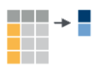
EXAMPLE 2: select columns

To get a sense for the code structure, let’s explore a couple verbs together. To start, let’s simplify our dataset to include only some variables of interest. Specifically, select() only the columns relevant to state names, county names, and the 2020 and 2016 Democratic support:

# What's the first argument? The second?
select(elections, c(state_name, county_name, dem_pct_20, dem_pct_16))

Let’s re-do this with the pipe function %>%:

elections %>% 
  select(state_name, county_name, dem_pct_20, dem_pct_16)

THE PIPE FUNCTION

%>% “passes” objects, usually datasets, to a function:

object %>% function() is the same function(object)

It improves code communication and human readability. For example, if we have many functions we want to use,

object %>% function() %>% function2() is the same function2(function(object))

The %>% like saying “and then” in English.

Note: You may see others use |> in R as the pipe. Both work in the same way.

EXAMPLE 3: filter rows

Let’s filter() out only the rows related to Minnesota (MN):

# Without a pipe
filter(elections, state_name == "Minnesota")

# With a pipe
elections %>% 
  filter(state_name == "Minnesota")

SUBTLETIES: == vs =

We use a == b to check whether a matches exactly b.

We use a = b to define that a is equal to b. We typically use = for this purpose inside a function, and <- for this purpose outside a function.

# Ex: "=" defines x
x = 2
x
## [1] 2

# Ex: "==" checks whether x is/matches 3
x == 3
## [1] FALSE

EXAMPLE 4: filter and select

Let’s combine select() and filter() to create a new dataset with info about the county names, and 2020 and 2016 Democratic support among Minnesota counties.

# Without pipes
filter(select(elections, c(state_name, county_name, dem_pct_20, dem_pct_16)), state_name == "Minnesota")

# With pipes: all verbs in 1 row
elections %>% select(state_name, county_name, dem_pct_20, dem_pct_16) %>% filter(state_name == "Minnesota")

# With pipes: each verb in a new row
elections %>% 
  select(state_name, county_name, dem_pct_20, dem_pct_16) %>% 
  filter(state_name == "Minnesota")

# We can even do this with UNtidyverse code in "base" R
elections[elections$state_name == "Minnesota", c(1, 4, 8, 12)]

REFLECT:

Why will we typically use:

tidyverse code
the pipe function %>%
each verb on a new row

EXAMPLE 5: order of operations

Sometimes, the order of operations matters. For example: putting on socks, then shoes produces a different result than putting on shoes, then socks. Sometimes order doesn’t matter. For example: Pouring cereal into a bowl, then adding milk produces the same result as pouring milk into a bowl, then adding cereal (though one order is obviously better than the other ;)) Above, we selected some columns and then filtered some rows:

elections %>% 
  select(state_name, county_name, dem_pct_20, dem_pct_16) %>% 
  filter(state_name == "Minnesota")

Would we get the same result if we reversed select() and filter()? Think first, then try it.

# Try it

EXAMPLE 6: Storing the results

Typically:

We want to store our data wrangling results.
It’s good practice to do so under a new name. We want to preserve, thus don’t want to overwrite, the original data (especially if our code contains errors!!).

# Store the results
mn <- elections %>% 
  select(state_name, county_name, dem_pct_20, dem_pct_16) %>% 
  filter(state_name == "Minnesota")

# Always check it out to confirm it's what you want it to be!
head(mn)
##   state_name      county_name dem_pct_20 dem_pct_16
## 1  Minnesota    Aitkin County      35.98      34.12
## 2  Minnesota     Anoka County      47.79      41.01
## 3  Minnesota    Becker County      33.96      30.47
## 4  Minnesota  Beltrami County      47.24      40.76
## 5  Minnesota    Benton County      32.70      28.33
## 6  Minnesota Big Stone County      35.41      33.75
nrow(mn)
## [1] 87
nrow(elections)
## [1] 3109

8.3 Exercises

GOALS

Learn, practice, and identify when to use the 6 wrangling verbs: select, mutate, filter, arrange, summarize, group_by.

DIRECTIONS

Work together.
Use the pipe function %>%.

Exercise 1: select practice

6 verbs: select, filter, arrange, mutate, summarize, group_by

Use select() to create a simplified dataset that we’ll use throughout the exercises below.

Store this dataset as elections_small.
Only keep the following variables: state_name, county_name, total_votes_20, repub_pct_20, dem_pct_20, total_votes_16, dem_pct_16

# Define elections_small
#___ <- ___ %>%
#  ___(___)

# Check out the first 6 rows to confirm your code did what you think it did!

Exercise 2: filter demo

6 verbs: select, filter, arrange, mutate, summarize, group_by

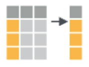
Whereas select() selects certain variables or columns, filter() keeps certain units of observation or rows relative to their outcome on certain variables. To this end, we must:

Identify the variable(s) that are relevant to the filter.
Use a “logical comparison operator” to define which values of the variable to keep:

symbol meaning

== equal to

!= not equal to

> greater than

>= greater than or equal to

< less than

<= less than or equal to

%in% c(???, ???) a list of multiple values
Use quotes “” when specifying outcomes of interest for a categorical variable.

symbol	meaning
==	equal to
!=	not equal to
>	greater than
>=	greater than or equal to
<	less than
<=	less than or equal to
%in% c(???, ???)	a list of multiple values

# Keep only data on counties in Hawaii
#elections_small %>% 
#  filter(___ ___ ___)

# What does this do?
elections_small %>% 
  filter(state_name %in% c("Hawaii", "Delaware"))
##   state_name       county_name total_votes_20 repub_pct_20 dem_pct_20
## 1   Delaware       Kent County          87025        47.12      51.19
## 2   Delaware New Castle County         287633        30.72      67.81
## 3   Delaware     Sussex County         129352        55.07      43.82
## 4     Hawaii     Hawaii County          87814        30.63      66.88
## 5     Hawaii   Honolulu County         382114        35.66      62.51
## 6     Hawaii      Kauai County          33497        34.58      63.36
## 7     Hawaii       Maui County          71044        31.14      66.59
##   total_votes_16 dem_pct_16
## 1          74253      44.91
## 2         261468      62.30
## 3         105814      37.17
## 4          64865      63.61
## 5         285683      61.48
## 6          26335      62.49
## 7          51942      64.45

# Keep only data on counties where the Republican got MORE THAN 93.97% of the vote in 2020
# THINK: What variable is relevant here?

# Keep only data on counties where the Republican got AT LEAST 93.97% of the vote in 2020
# This should have 1 more row than your answer above

We can also filter with respect to 2 rules! Here, think what variables are relevant.

# Keep only data on counties in Texas where the Democrat got more than 65% of the vote in 2020
# Do this 2 ways.
# Method 1: 2 filters with 1 condition each
#elections_small %>% 
#  filter(___) %>% 
#  filter(___)

# Method 2: 1 filter with 2 conditions
#elections_small %>% 
#  filter(___, ___)

Exercise 3: arrange demo

6 verbs: select, filter, arrange, mutate, summarize, group_by

arrange() arranges or sorts the rows in a dataset according to a given column or variable, in ascending or descending order:

arrange(variable), arrange(desc(variable))

# Arrange the counties in elections_small from lowest to highest percentage of 2020 Republican support
# Print out just the first 6 rows
# elections_small %>% 
#   arrange(___) %>% 
#   head()

# Arrange the counties in elections_small from highest to lowest percentage of 2020 Republican support
# Print out just the first 6 rows

Exercise 4: mutate demo

6 verbs: select, filter, arrange, mutate, summarize, group_by

mutate() can either transform / mutate an existing variable (column), or define a new variable based on existing ones.

Part a

# What did this code do?
elections_small %>% 
  mutate(diff_20 = repub_pct_20 - dem_pct_20) %>% 
  head()
##   state_name    county_name total_votes_20 repub_pct_20 dem_pct_20
## 1    Alabama Autauga County          27770        71.44      27.02
## 2    Alabama Baldwin County         109679        76.17      22.41
## 3    Alabama Barbour County          10518        53.45      45.79
## 4    Alabama    Bibb County           9595        78.43      20.70
## 5    Alabama  Blount County          27588        89.57       9.57
## 6    Alabama Bullock County           4613        24.84      74.70
##   total_votes_16 dem_pct_16 diff_20
## 1          24661      23.96   44.42
## 2          94090      19.57   53.76
## 3          10390      46.66    7.66
## 4           8748      21.42   57.73
## 5          25384       8.47   80.00
## 6           4701      75.09  -49.86

# What did this code do?
elections_small %>% 
  mutate(repub_votes_20 = round(total_votes_20 * repub_pct_20/100)) %>% 
  head()
##   state_name    county_name total_votes_20 repub_pct_20 dem_pct_20
## 1    Alabama Autauga County          27770        71.44      27.02
## 2    Alabama Baldwin County         109679        76.17      22.41
## 3    Alabama Barbour County          10518        53.45      45.79
## 4    Alabama    Bibb County           9595        78.43      20.70
## 5    Alabama  Blount County          27588        89.57       9.57
## 6    Alabama Bullock County           4613        24.84      74.70
##   total_votes_16 dem_pct_16 repub_votes_20
## 1          24661      23.96          19839
## 2          94090      19.57          83542
## 3          10390      46.66           5622
## 4           8748      21.42           7525
## 5          25384       8.47          24711
## 6           4701      75.09           1146

# What did this code do?
elections_small %>% 
  mutate(repub_win_20 = repub_pct_20 > dem_pct_20) %>% 
  head()
##   state_name    county_name total_votes_20 repub_pct_20 dem_pct_20
## 1    Alabama Autauga County          27770        71.44      27.02
## 2    Alabama Baldwin County         109679        76.17      22.41
## 3    Alabama Barbour County          10518        53.45      45.79
## 4    Alabama    Bibb County           9595        78.43      20.70
## 5    Alabama  Blount County          27588        89.57       9.57
## 6    Alabama Bullock County           4613        24.84      74.70
##   total_votes_16 dem_pct_16 repub_win_20
## 1          24661      23.96         TRUE
## 2          94090      19.57         TRUE
## 3          10390      46.66         TRUE
## 4           8748      21.42         TRUE
## 5          25384       8.47         TRUE
## 6           4701      75.09        FALSE

Part b

# You try
# Define a variable that calculates the change in Dem support in 2020 vs 2016
#elections_small %>% 
#  mutate(_____) %>% 
#  head()

# You try
# Define a variable that determines whether the Dem support was higher in 2020 than in 2016 (TRUE/FALSE)
#elections_small %>% 
#  mutate(_____) %>% 
#  head()

Exercise 5: Pipe series

Let’s now combine these verbs into a pipe series!

Part a

IMPORTANT: BEFORE running the below chunk, what do you think it will produce?

elections_small %>% 
  filter(state_name == "Wisconsin",
         repub_pct_20 < dem_pct_20) %>% 
  arrange(desc(total_votes_20)) %>% 
  head()
##   state_name       county_name total_votes_20 repub_pct_20 dem_pct_20
## 1  Wisconsin  Milwaukee County         458971        29.27      69.13
## 2  Wisconsin       Dane County         344791        22.85      75.46
## 3  Wisconsin       Rock County          85360        43.51      54.66
## 4  Wisconsin  La Crosse County          67884        42.25      55.75
## 5  Wisconsin Eau Claire County          58275        43.49      54.26
## 6  Wisconsin    Portage County          40603        47.53      50.31
##   total_votes_16 dem_pct_16
## 1         434970      66.44
## 2         304729      71.38
## 3          75043      52.42
## 4          62785      51.61
## 5          54080      50.43
## 6          38123      48.59

Part b

IMPORTANT: BEFORE trying, what do you think will happen if you change the order of filter and arrange:

the results will be the same
we’ll get an error
we won’t get an error, but the results will be different

# Now try it. Change the order of filter and arrange below.
elections_small %>% 
  filter(state_name == "Wisconsin",
         repub_pct_20 < dem_pct_20) %>% 
  arrange(desc(total_votes_20)) %>% 
  head()
##   state_name       county_name total_votes_20 repub_pct_20 dem_pct_20
## 1  Wisconsin  Milwaukee County         458971        29.27      69.13
## 2  Wisconsin       Dane County         344791        22.85      75.46
## 3  Wisconsin       Rock County          85360        43.51      54.66
## 4  Wisconsin  La Crosse County          67884        42.25      55.75
## 5  Wisconsin Eau Claire County          58275        43.49      54.26
## 6  Wisconsin    Portage County          40603        47.53      50.31
##   total_votes_16 dem_pct_16
## 1         434970      66.44
## 2         304729      71.38
## 3          75043      52.42
## 4          62785      51.61
## 5          54080      50.43
## 6          38123      48.59

Part c

So the order of filter() and arrange() did not matter – rerranging them produces the same results. BUT what is one advantage of filtering before arranging?

Part d

IMPORTANT: BEFORE running the below chunk, what do you think it will produce?

elections_small %>% 
  filter(state_name == "Delaware") %>% 
  mutate(repub_win_20 = repub_pct_20 > dem_pct_20) %>% 
  select(county_name, repub_pct_20, dem_pct_20, repub_win_20)
##         county_name repub_pct_20 dem_pct_20 repub_win_20
## 1       Kent County        47.12      51.19        FALSE
## 2 New Castle County        30.72      67.81        FALSE
## 3     Sussex County        55.07      43.82         TRUE

Part e

IMPORTANT: BEFORE trying, what do you think will happen if you change the order of mutate and select:

the results will be the same
we’ll get an error
we won’t get an error, but the results will be different

# Now try it. Change the order of mutate and select below.
elections_small %>% 
  filter(state_name == "Delaware") %>% 
  mutate(repub_win_20 = repub_pct_20 > dem_pct_20) %>% 
  select(county_name, repub_pct_20, dem_pct_20, repub_win_20)
##         county_name repub_pct_20 dem_pct_20 repub_win_20
## 1       Kent County        47.12      51.19        FALSE
## 2 New Castle County        30.72      67.81        FALSE
## 3     Sussex County        55.07      43.82         TRUE

Exercise 6: DIY pipe series

We’ve now learned 4 of the 6 wrangling verbs: select, filter, mutate, arrange. Let’s practice combining these into pipe series. Here are some hot tips:

Before writing any code, translate the prompt: how many distinct wrangling steps are needed and what verb do we need in each step?
Add each verb one at a time – don’t try writing a whole chunk at once.

Part a

Show just the counties in Minnesota and their Democratic 2020 vote percentage, from highest to lowest. Your answer should have just 2 columns.

Part b

Create a new dataset named mn_wi that sorts the counties in Minnesota and Wisconsin from lowest to highest in terms of the change in Democratic vote percentage in 2020 vs 2016. This dataset should include the following variables (and only these variables): state_name, county_name, dem_pct_20, dem_pct_16, and a variable measuring the change in Democratic vote percentage in 2020 vs 2016.

# Define the dataset
# Only store the results once you're confident that they're correct


# Check out the first 6 rows to confirm your results

Part c

Construct and discuss a plot of the county-level change in Democratic vote percent in 2020 vs 2016, and how this differs between Minnesota and Wisconsin.

Exercise 7: summarize demo

6 verbs: select, filter, arrange, mutate, summarize, group_by

Let’s talk about the last 2 verbs. summarize() (or equivalently summarise()) takes an entire data frame as input and outputs a single row with one or more summary statistics. For each chunk below, indicate what the code does.

# What does this do?
elections_small %>% 
  summarize(median(repub_pct_20))
##   median(repub_pct_20)
## 1                68.29

# What does this do?
elections_small %>% 
  summarize(median_repub = median(repub_pct_20))
##   median_repub
## 1        68.29

# What does this do?
elections_small %>% 
  summarize(median_repub = median(repub_pct_20), total_votes = sum(total_votes_20))
##   median_repub total_votes
## 1        68.29   157949293

Exercise 8: `summarize` + `group_by` demo

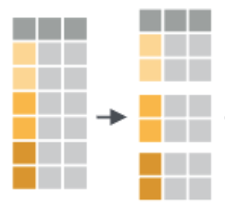
6 verbs: select, filter, arrange, mutate, summarize, group_by

Finally, group_by() groups the units of observation or rows of a data frame by a specified set of variables. Alone, this function doesn’t change the appearance of our dataset or seem to do anything at all:

elections_small %>% 
  group_by(state_name) %>% 
  head()
## # A tibble: 6 × 7
## # Groups:   state_name [1]
##   state_name county_name   total_votes_20 repub_pct_20 dem_pct_20 total_votes_16
##   <chr>      <chr>                  <int>        <dbl>      <dbl>          <int>
## 1 Alabama    Autauga Coun…          27770         71.4      27.0           24661
## 2 Alabama    Baldwin Coun…         109679         76.2      22.4           94090
## 3 Alabama    Barbour Coun…          10518         53.4      45.8           10390
## 4 Alabama    Bibb County             9595         78.4      20.7            8748
## 5 Alabama    Blount County          27588         89.6       9.57          25384
## 6 Alabama    Bullock Coun…           4613         24.8      74.7            4701
## # ℹ 1 more variable: dem_pct_16 <dbl>

Though it does change the underlying structure of the dataset:

# Check out the structure before and after group_by
elections_small %>% 
  class()
## [1] "data.frame"

elections_small %>% 
  group_by(state_name) %>% 
  class()
## [1] "grouped_df" "tbl_df"     "tbl"        "data.frame"

Where it really shines is in partnership with summarize().

# What does this do?
# (What if we didn't use group_by?)
elections_small %>% 
  group_by(state_name) %>% 
  summarize(median_repub = median(repub_pct_20), total_votes = sum(total_votes_20)) 
## # A tibble: 50 × 3
##    state_name           median_repub total_votes
##    <chr>                       <dbl>       <int>
##  1 Alabama                      70.6     2323304
##  2 Arizona                      57.9     3387326
##  3 Arkansas                     72.1     1219069
##  4 California                   44.8    17495906
##  5 Colorado                     56.2     3256953
##  6 Connecticut                  41.0     1824280
##  7 Delaware                     47.1      504010
##  8 District of Columbia          5.4      344356
##  9 Florida                      64.6    11067456
## 10 Georgia                      68       4997716
## # ℹ 40 more rows

REFLECT:
Notice that group_by() with summarize() produces new data frame or tibble! But the units of observation are now states instead of counties within states.

Exercise 9: DIY

Let’s practice (some of) our 6 verbs: select, filter, arrange, mutate, summarize, group_by Remember:

Before writing any code, translate the given prompts: how many distinct wrangling steps are needed and what verb do we need in each step?
Add each verb one at a time.

Part a

NOTE: Part a is a challenge exercise. If you get really stuck, move on to Part b which is the same overall question, but with hints.

# Sort the *states* from the most to least total votes cast in 2020

# In 2020, what were the total number of votes for the Democratic candidate and the total number of votes for the Republican candidate in each *state*?

# What states did the Democratic candidate win in 2020?

Part b

# Sort the states from the most to least total votes cast in 2020
# HINT: Calculate the total number of votes in each state, then sort

# In 2020, what were the total number of votes for the Democratic candidate and the total number of votes for the Republican candidate in each state?
# HINT: First calculate the number of Dem and Repub votes in each *county*
# Then group and summarize these by state

# What states did the Democratic candidate win in 2020?
# HINT: Start with the results from the previous chunk, and then keep only some rows

Exercise 10: Practice on new data

Recall the World Cup football/soccer data from TidyTuesday:

world_cup <- read.csv("https://raw.githubusercontent.com/rfordatascience/tidytuesday/master/data/2022/2022-11-29/worldcups.csv")

You can find a codebook here. Use (some of) our 6 verbs (select, filter, arrange, mutate, summarize, group_by) and data viz to address the following prompts.

# In what years did Brazil win the World Cup?

# What were the 6 World Cups with the highest attendance?

# Construct a univariate plot of goals_scored (no wrangling necessary)
# This provides a visual summary of how the number of goals_scored varies from World Cup to World Cup

# Let's follow up the plot with some more precise numerical summaries
# Calculate the min, median, and max number of goals_scored across all World Cups
# NOTE: Visually compare these numerical summaries to what you observed in the plot

# Construct a bivariate plot of how the number of goals_scored in the World Cup has changed over the years
# No wrangling necessary

# Our above summaries might be a bit misleading.
# The number of games played at the World Cup varies.
# Construct a bivariate plot of how the typical number of goals per game has changed over the years

Exercise 11: More viz review

Let’s re-consider Minnesota and Wisconsin. Use mn_wi_new throughout this exercise to practice identifying what viz is appropriate in a given situation, and how to create that viz.

Challenge yourself to not just start typing things until something works – first think about what plot would be appropriate.

mn_wi_new <- elections %>%
  filter(state_name %in% c("Minnesota", "Wisconsin")) %>%
  mutate(repub_win_20 = (repub_pct_20 > dem_pct_20),
          repub_win_16 = (repub_pct_16 > dem_pct_16),
          ) %>%
  select(state_abbr, repub_pct_20, repub_pct_16, repub_pct_12, repub_win_20, repub_win_16)
head(mn_wi_new)
##   state_abbr repub_pct_20 repub_pct_16 repub_pct_12 repub_win_20 repub_win_16
## 1         MN        62.42        60.05        49.76         TRUE         TRUE
## 2         MN        49.69        50.71        50.31         TRUE         TRUE
## 3         MN        64.11        63.66        56.37         TRUE         TRUE
## 4         MN        50.39        50.59        43.91         TRUE         TRUE
## 5         MN        64.61        64.65        55.58         TRUE         TRUE
## 6         MN        62.64        58.89        49.77         TRUE         TRUE

# Construct a plot that illustrates the relationship of  repub_pct_20 with repub_pct_16 and repub_pct_12

# Construct a plot that illustrates the relationship of  repub_pct_20 with repub_pct_16 in MN vs WI.
# Do this in 1 frame and add a linear trend

# Construct a plot that illustrates the relationship of  repub_pct_20 with repub_pct_16 in MN vs WI.
# Do this in 2 separate frames -- 1 for MN and 1 for WI
# and include linear trends

# Construct a plot that illustrates how many counties were
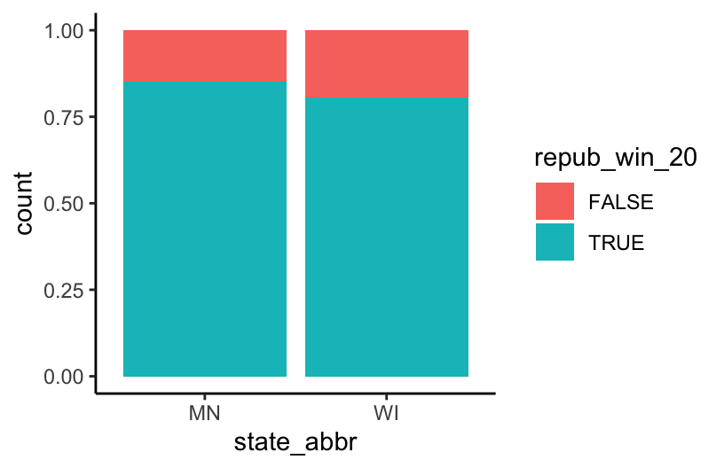
# won by the republican in 2020, combining MN and WI counties

# Construct a plot that illustrates how many counties were
# won by the republican in 2020 in MN vs WI, i.e.
# the relationship between state_abbr and repub_win_20

# Starting with the previous plot, and if you didn't already,
# tweak it so that we can directly compare the proportion
# of counties won by the republican in 2020 in MN and WI,
# ignoring the fact that MN has more counties

8.4 Wrap-up

Homework 3 is due tonight!
Quiz 1 is next Tuesday. It won’t cover material from today.
Make sure to complete any exercises from today’s activity before our next class.
Reach out on Slack, in office hours, etc.

:::

8.5 Solutions

Click for Solutions

8.5.1 EXAMPLE 1

select
filter
mutate
arrange
summarize

Exercise 1: select practice

# Define elections_small
elections_small <- elections %>%
  select(state_name, county_name, total_votes_20, repub_pct_20, dem_pct_20, total_votes_16, dem_pct_16)

# Check out the first 6 rows to confirm your code did what you think it did!
head(elections_small)
##   state_name    county_name total_votes_20 repub_pct_20 dem_pct_20
## 1    Alabama Autauga County          27770        71.44      27.02
## 2    Alabama Baldwin County         109679        76.17      22.41
## 3    Alabama Barbour County          10518        53.45      45.79
## 4    Alabama    Bibb County           9595        78.43      20.70
## 5    Alabama  Blount County          27588        89.57       9.57
## 6    Alabama Bullock County           4613        24.84      74.70
##   total_votes_16 dem_pct_16
## 1          24661      23.96
## 2          94090      19.57
## 3          10390      46.66
## 4           8748      21.42
## 5          25384       8.47
## 6           4701      75.09

Exercise 2: filter demo

# Keep only data on counties in Hawaii
elections_small %>%
 filter(state_name == "Hawaii")
##   state_name     county_name total_votes_20 repub_pct_20 dem_pct_20
## 1     Hawaii   Hawaii County          87814        30.63      66.88
## 2     Hawaii Honolulu County         382114        35.66      62.51
## 3     Hawaii    Kauai County          33497        34.58      63.36
## 4     Hawaii     Maui County          71044        31.14      66.59
##   total_votes_16 dem_pct_16
## 1          64865      63.61
## 2         285683      61.48
## 3          26335      62.49
## 4          51942      64.45

# Keep counties in Hawaii AND Delaware
elections_small %>% 
  filter(state_name %in% c("Hawaii", "Delaware"))
##   state_name       county_name total_votes_20 repub_pct_20 dem_pct_20
## 1   Delaware       Kent County          87025        47.12      51.19
## 2   Delaware New Castle County         287633        30.72      67.81
## 3   Delaware     Sussex County         129352        55.07      43.82
## 4     Hawaii     Hawaii County          87814        30.63      66.88
## 5     Hawaii   Honolulu County         382114        35.66      62.51
## 6     Hawaii      Kauai County          33497        34.58      63.36
## 7     Hawaii       Maui County          71044        31.14      66.59
##   total_votes_16 dem_pct_16
## 1          74253      44.91
## 2         261468      62.30
## 3         105814      37.17
## 4          64865      63.61
## 5         285683      61.48
## 6          26335      62.49
## 7          51942      64.45

# Keep only data on counties where the Republican got MORE THAN 93.97% of the vote in 2020
elections_small %>% 
  filter(repub_pct_20 > 93.97)
##   state_name    county_name total_votes_20 repub_pct_20 dem_pct_20
## 1      Texas  Borden County            416        95.43       3.85
## 2      Texas    King County            159        94.97       5.03
## 3      Texas Roberts County            550        96.18       3.09
##   total_votes_16 dem_pct_16
## 1            365       8.49
## 2            159       3.14
## 3            550       3.64

# Keep only data on counties where the Republican got AT LEAST 93.97% of the vote in 2020
# This should have 1 more row than your answer above
elections_small %>% 
  filter(repub_pct_20 >= 93.97)
##   state_name     county_name total_votes_20 repub_pct_20 dem_pct_20
## 1    Montana Garfield County            813        93.97       5.04
## 2      Texas   Borden County            416        95.43       3.85
## 3      Texas     King County            159        94.97       5.03
## 4      Texas  Roberts County            550        96.18       3.09
##   total_votes_16 dem_pct_16
## 1            715       4.76
## 2            365       8.49
## 3            159       3.14
## 4            550       3.64

# Keep only data on counties in Texas where the Democrat got more than 65% of the vote in 2020
# Do this 2 ways.
# Method 1: 2 filters with 1 condition each
elections_small %>%
 filter(state_name == "Texas") %>%
 filter(dem_pct_20 > 65)
##   state_name     county_name total_votes_20 repub_pct_20 dem_pct_20
## 1      Texas  El Paso County         267215        31.56      66.66
## 2      Texas Presidio County           2217        32.52      65.99
## 3      Texas   Travis County         610349        26.43      71.41
## 4      Texas   Zavala County           4379        34.03      65.40
##   total_votes_16 dem_pct_16
## 1         210458      69.14
## 2           2203      66.18
## 3         462511      66.26
## 4           3390      77.67

# Method 2: 1 filter with 2 conditions
elections_small %>%
 filter(state_name == "Texas", dem_pct_20 > 65)
##   state_name     county_name total_votes_20 repub_pct_20 dem_pct_20
## 1      Texas  El Paso County         267215        31.56      66.66
## 2      Texas Presidio County           2217        32.52      65.99
## 3      Texas   Travis County         610349        26.43      71.41
## 4      Texas   Zavala County           4379        34.03      65.40
##   total_votes_16 dem_pct_16
## 1         210458      69.14
## 2           2203      66.18
## 3         462511      66.26
## 4           3390      77.67

Exercise 3: arrange demo

# Arrange the counties in elections_small from lowest to highest percentage of 2020 Republican support
# Print out just the first 6 rows
elections_small %>%
  arrange(repub_pct_20) %>%
  head()
##             state_name            county_name total_votes_20 repub_pct_20
## 1 District of Columbia   District of Columbia         344356         5.40
## 2             Maryland Prince George's County         424855         8.73
## 3             Maryland         Baltimore city         237461        10.69
## 4             Virginia        Petersburg city          14118        11.22
## 5             New York        New York County         694904        12.26
## 6           California   San Francisco County         443458        12.72
##   dem_pct_20 total_votes_16 dem_pct_16
## 1      92.15         280272      92.85
## 2      89.26         351091      89.33
## 3      87.28         208980      85.44
## 4      87.75          13717      87.52
## 5      86.78         591368      87.17
## 6      85.27         365295      85.53

# Arrange the counties in elections_small from highest to lowest percentage of 2020 Republican support
# Print out just the first 6 rows
elections_small %>%
  arrange(desc(repub_pct_20)) %>%
  head()
##   state_name      county_name total_votes_20 repub_pct_20 dem_pct_20
## 1      Texas   Roberts County            550        96.18       3.09
## 2      Texas    Borden County            416        95.43       3.85
## 3      Texas      King County            159        94.97       5.03
## 4    Montana  Garfield County            813        93.97       5.04
## 5      Texas Glasscock County            653        93.57       5.97
## 6   Nebraska     Grant County            402        93.28       4.98
##   total_votes_16 dem_pct_16
## 1            550       3.64
## 2            365       8.49
## 3            159       3.14
## 4            715       4.76
## 5            602       5.65
## 6            394       5.08

Exercise 4: mutate demo

# Define diff_20, the difference btwn the Repub and Dem percent in 2020
elections_small %>% 
  mutate(diff_20 = repub_pct_20 - dem_pct_20) %>% 
  head()
##   state_name    county_name total_votes_20 repub_pct_20 dem_pct_20
## 1    Alabama Autauga County          27770        71.44      27.02
## 2    Alabama Baldwin County         109679        76.17      22.41
## 3    Alabama Barbour County          10518        53.45      45.79
## 4    Alabama    Bibb County           9595        78.43      20.70
## 5    Alabama  Blount County          27588        89.57       9.57
## 6    Alabama Bullock County           4613        24.84      74.70
##   total_votes_16 dem_pct_16 diff_20
## 1          24661      23.96   44.42
## 2          94090      19.57   53.76
## 3          10390      46.66    7.66
## 4           8748      21.42   57.73
## 5          25384       8.47   80.00
## 6           4701      75.09  -49.86

# Define repub_votes_20, the number (not percent) of Repub votes in 2020
elections_small %>% 
  mutate(repub_votes_20 = round(total_votes_20 * repub_pct_20/100)) %>% 
  head()
##   state_name    county_name total_votes_20 repub_pct_20 dem_pct_20
## 1    Alabama Autauga County          27770        71.44      27.02
## 2    Alabama Baldwin County         109679        76.17      22.41
## 3    Alabama Barbour County          10518        53.45      45.79
## 4    Alabama    Bibb County           9595        78.43      20.70
## 5    Alabama  Blount County          27588        89.57       9.57
## 6    Alabama Bullock County           4613        24.84      74.70
##   total_votes_16 dem_pct_16 repub_votes_20
## 1          24661      23.96          19839
## 2          94090      19.57          83542
## 3          10390      46.66           5622
## 4           8748      21.42           7525
## 5          25384       8.47          24711
## 6           4701      75.09           1146

# Define repub_win_20, whether the Repub won in 2020 (TRUE or FALSE!)
elections_small %>% 
  mutate(repub_win_20 = repub_pct_20 > dem_pct_20) %>% 
  head()
##   state_name    county_name total_votes_20 repub_pct_20 dem_pct_20
## 1    Alabama Autauga County          27770        71.44      27.02
## 2    Alabama Baldwin County         109679        76.17      22.41
## 3    Alabama Barbour County          10518        53.45      45.79
## 4    Alabama    Bibb County           9595        78.43      20.70
## 5    Alabama  Blount County          27588        89.57       9.57
## 6    Alabama Bullock County           4613        24.84      74.70
##   total_votes_16 dem_pct_16 repub_win_20
## 1          24661      23.96         TRUE
## 2          94090      19.57         TRUE
## 3          10390      46.66         TRUE
## 4           8748      21.42         TRUE
## 5          25384       8.47         TRUE
## 6           4701      75.09        FALSE

Exercise 5: Pipe series

Part c

It’s more “computationally efficient” to get rid of some rows before arranging.

Part e

We can’t select a variable before we define it!

Exercise 6: DIY pipe series

Part a

Here’s my translation:

just the counties in Minnesota —> filter
just the counties in Minnesota and their Democratic 2020 vote percentage —> select
from highest to lowest —> arrange

# Remember to try this 1 line at a time
elections_small %>% 
  filter(state_name == "Minnesota") %>% 
  select(county_name, dem_pct_20) %>% 
  arrange(desc(dem_pct_20))
##                 county_name dem_pct_20
## 1             Ramsey County      71.50
## 2           Hennepin County      70.46
## 3               Cook County      65.58
## 4          St. Louis County      56.64
## 5             Dakota County      55.73
## 6            Olmsted County      54.16
## 7         Washington County      53.46
## 8         Blue Earth County      50.84
## 9               Clay County      50.74
## 10              Lake County      50.64
## 11          Nicollet County      50.31
## 12           Carlton County      49.58
## 13            Winona County      49.07
## 14              Rice County      48.76
## 15          Mahnomen County      48.26
## 16             Anoka County      47.79
## 17          Beltrami County      47.24
## 18            Carver County      46.37
## 19             Mower County      46.00
## 20             Scott County      45.52
## 21           Houston County      42.42
## 22           Goodhue County      41.23
## 23          Freeborn County      40.96
## 24            Norman County      40.80
## 25            Itasca County      40.61
## 26       Koochiching County      38.41
## 27          Watonwan County      38.20
## 28           Kittson County      38.12
## 29           Stevens County      37.80
## 30           Stearns County      37.58
## 31          Fillmore County      37.48
## 32            Steele County      37.47
## 33         Kandiyohi County      36.12
## 34            Aitkin County      35.98
## 35              Lyon County      35.94
## 36     Lac qui Parle County      35.79
## 37           Wabasha County      35.78
## 38             Grant County      35.58
## 39          Traverse County      35.46
## 40         Big Stone County      35.41
## 41        Pennington County      35.29
## 42              Pope County      35.27
## 43              Polk County      34.88
## 44              Cass County      34.68
## 45            Wright County      34.49
## 46           Hubbard County      34.42
## 47             Swift County      34.35
## 48         Crow Wing County      34.17
## 49           Chisago County      34.15
## 50            Becker County      33.96
## 51              Pine County      33.87
## 52          Le Sueur County      33.73
## 53          Chippewa County      33.67
## 54            Nobles County      33.65
## 55            Waseca County      33.65
## 56             Dodge County      33.47
## 57        Otter Tail County      32.85
## 58            Benton County      32.70
## 59           Douglas County      32.56
## 60             Brown County      32.48
## 61         Sherburne County      32.48
## 62         Faribault County      31.98
## 63          Red Lake County      31.47
## 64          Renville County      30.71
## 65            McLeod County      30.64
## 66   Yellow Medicine County      30.54
## 67           Lincoln County      30.08
## 68        Cottonwood County      30.03
## 69           Kanabec County      30.02
## 70            Martin County      30.02
## 71           Jackson County      29.99
## 72        Mille Lacs County      29.98
## 73            Wilkin County      29.91
## 74              Rock County      29.69
## 75            Murray County      29.60
## 76            Isanti County      29.45
## 77            Sibley County      28.60
## 78            Meeker County      28.58
## 79           Redwood County      28.43
## 80 Lake of the Woods County      27.87
## 81        Clearwater County      26.76
## 82         Pipestone County      26.44
## 83            Wadena County      26.35
## 84            Roseau County      25.98
## 85          Marshall County      25.33
## 86              Todd County      24.79
## 87          Morrison County      22.33

Part b

Here’s my translation:

counties in Minnesota and Wisconsin —> filter
change in Democratic vote percentage in 2020 vs 2016 —> mutate (we don’t already have this)
sorts the counties from highest to lowest —> arrange
include the following variables (and only these variables) —> select

# Remember to try this 1 line at a time before storing!
mn_wi <- elections_small %>% 
  filter(state_name %in% c("Minnesota", "Wisconsin")) %>% 
  select(state_name, county_name, dem_pct_20, dem_pct_16) %>%
  mutate(dem_change = dem_pct_20 - dem_pct_16) %>% 
  arrange(dem_change)
  
# Check it out
head(mn_wi)
##   state_name        county_name dem_pct_20 dem_pct_16 dem_change
## 1  Minnesota     Stevens County      37.80      39.55      -1.75
## 2  Wisconsin      Forest County      34.06      35.12      -1.06
## 3  Wisconsin    Kewaunee County      32.87      33.73      -0.86
## 4  Wisconsin       Clark County      30.37      31.19      -0.82
## 5  Wisconsin       Adams County      36.63      37.40      -0.77
## 6  Wisconsin Trempealeau County      40.86      41.57      -0.71

Part c

There was a stronger Dem shift from 2016 to 2020 in Minnesota. Further, in most counties across both states, the percent Dem tended to be higher in 2020 than in 2016.

ggplot(mn_wi, aes(x = dem_change, fill = state_name)) + 
  geom_density(alpha = 0.5)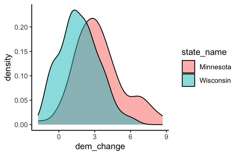

ggplot(mn_wi, aes(y = dem_change, x = state_name)) + 
  geom_boxplot()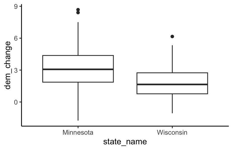

Exercise 7: summarize demo

# Calculate the median Repub vote percentage in 2020 across all counties
elections_small %>% 
  summarize(median(repub_pct_20))
##   median(repub_pct_20)
## 1                68.29

# Calculate the median Repub vote percentage in 2020 across all counties
# AND name it "median_repub"
elections_small %>% 
  summarize(median_repub = median(repub_pct_20))
##   median_repub
## 1        68.29

# Calculate the median Repub vote percentage in 2020 across all counties
# AND the total number of votes across all counties
# AND name the results
elections_small %>% 
  summarize(median_repub = median(repub_pct_20), total_votes = sum(total_votes_20))
##   median_repub total_votes
## 1        68.29   157949293

Exercise 8: `summarize` + `group_by` demo

# Calculate the median 2020 Repub percent and total votes BY STATE
elections_small %>% 
  group_by(state_name) %>% 
  summarize(median_repub = median(repub_pct_20), total_votes = sum(total_votes_20)) 
## # A tibble: 50 × 3
##    state_name           median_repub total_votes
##    <chr>                       <dbl>       <int>
##  1 Alabama                      70.6     2323304
##  2 Arizona                      57.9     3387326
##  3 Arkansas                     72.1     1219069
##  4 California                   44.8    17495906
##  5 Colorado                     56.2     3256953
##  6 Connecticut                  41.0     1824280
##  7 Delaware                     47.1      504010
##  8 District of Columbia          5.4      344356
##  9 Florida                      64.6    11067456
## 10 Georgia                      68       4997716
## # ℹ 40 more rows

Exercise 9: DIY

Part a

# Sort the states from the most to least total votes in 2020
elections_small %>% 
  group_by(state_name) %>% 
  summarize(total = sum(total_votes_20)) %>% 
  arrange(desc(total))
## # A tibble: 50 × 2
##    state_name        total
##    <chr>             <int>
##  1 California     17495906
##  2 Texas          11317911
##  3 Florida        11067456
##  4 New York        8616205
##  5 Pennsylvania    6925255
##  6 Illinois        6038850
##  7 Ohio            5922202
##  8 Michigan        5539302
##  9 North Carolina  5524801
## 10 Georgia         4997716
## # ℹ 40 more rows

# In 2020, what were the total number of votes for the Democratic candidate and the total number of votes for the Republican candidate in each *state*?
elections_small %>% 
  mutate(dem_votes_20 = round(total_votes_20 * dem_pct_20 / 100), 
         repub_votes_20 = round(total_votes_20 * repub_pct_20 / 100)) %>% 
  group_by(state_name) %>% 
  summarize(dem_total = sum(dem_votes_20),
            repub_total = sum(repub_votes_20))
## # A tibble: 50 × 3
##    state_name           dem_total repub_total
##    <chr>                    <dbl>       <dbl>
##  1 Alabama                 849664     1441155
##  2 Arizona                1672127     1661671
##  3 Arkansas                423919      760641
##  4 California            11109642     6006031
##  5 Colorado               1804393     1364627
##  6 Connecticut            1080677      715315
##  7 Delaware                296274      200601
##  8 District of Columbia    317324       18595
##  9 Florida                5297131     5668600
## 10 Georgia                2473661     2461869
## # ℹ 40 more rows

# What states did the Democratic candidate win in 2020?
elections_small %>% 
  mutate(dem_votes_20 = round(total_votes_20 * dem_pct_20 / 100), 
         repub_votes_20 = round(total_votes_20 * repub_pct_20 / 100)) %>% 
  group_by(state_name) %>% 
  summarize(dem_total = sum(dem_votes_20),
            repub_total = sum(repub_votes_20)) %>% 
  filter(dem_total > repub_total)
## # A tibble: 26 × 3
##    state_name           dem_total repub_total
##    <chr>                    <dbl>       <dbl>
##  1 Arizona                1672127     1661671
##  2 California            11109642     6006031
##  3 Colorado               1804393     1364627
##  4 Connecticut            1080677      715315
##  5 Delaware                296274      200601
##  6 District of Columbia    317324       18595
##  7 Georgia                2473661     2461869
##  8 Hawaii                  366121      196865
##  9 Illinois               3471916     2446931
## 10 Maine                   430466      359897
## # ℹ 16 more rows

Exercise 10: Practice on new data

# In what years did Brazil win the World Cup?
world_cup %>% 
  filter(winner == "Brazil")
##   year               host winner         second        third       fourth
## 1 1958             Sweden Brazil         Sweden       France West Germany
## 2 1962              Chile Brazil Czechoslovakia        Chile   Yugoslavia
## 3 1970             Mexico Brazil          Italy West Germany      Uruguay
## 4 1994                USA Brazil          Italy       Sweden     Bulgaria
## 5 2002 Japan, South Korea Brazil        Germany       Turkey  South Korea
##   goals_scored teams games attendance
## 1          126    16    35     868000
## 2           89    16    32     776000
## 3           95    16    32    1673975
## 4          141    24    52    3568567
## 5          161    32    64    2724604

# What were the 6 World Cups with the highest attendance?
world_cup %>% 
  arrange(desc(attendance)) %>% 
  head()
##   year               host  winner    second       third      fourth
## 1 1994                USA  Brazil     Italy      Sweden    Bulgaria
## 2 2014             Brazil Germany Argentina Netherlands      Brazil
## 3 2006            Germany   Italy    France     Germany    Portugal
## 4 2018             Russia  France   Croatia     Belgium     England
## 5 1998             France  France    Brazil     Croatia Netherlands
## 6 2002 Japan, South Korea  Brazil   Germany      Turkey South Korea
##   goals_scored teams games attendance
## 1          141    24    52    3568567
## 2          171    32    64    3441450
## 3          147    32    64    3367000
## 4          169    32    64    3031768
## 5          171    32    64    2859234
## 6          161    32    64    2724604

# Construct a univariate plot of goals_scored (no wrangling necessary)
# This provides a visual summary of how the number of goals_scored varies from World Cup to World Cup
ggplot(world_cup, aes(x = goals_scored)) + 
  geom_histogram(color = "white")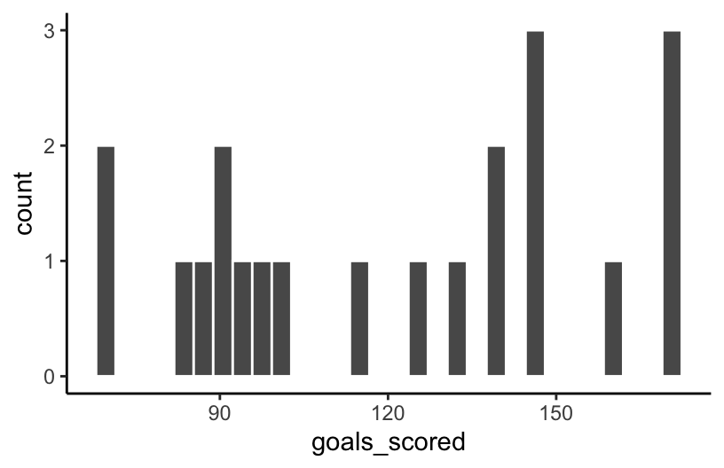

# Let's follow up the plot with some more precise numerical summaries
# Calculate the min, median, and max number of goals_scored across all World Cups
# NOTE: Visually compare these numerical summaries to what you observed in the plot
world_cup %>% 
  summarize(min(goals_scored), median(goals_scored), max(goals_scored))
##   min(goals_scored) median(goals_scored) max(goals_scored)
## 1                70                  126               171

# Construct a bivariate plot of how the number of goals_scored in the World Cup has changed over the years
# No wrangling necessary
ggplot(world_cup, aes(x = year, y = goals_scored)) + 
  geom_point() + 
  geom_line()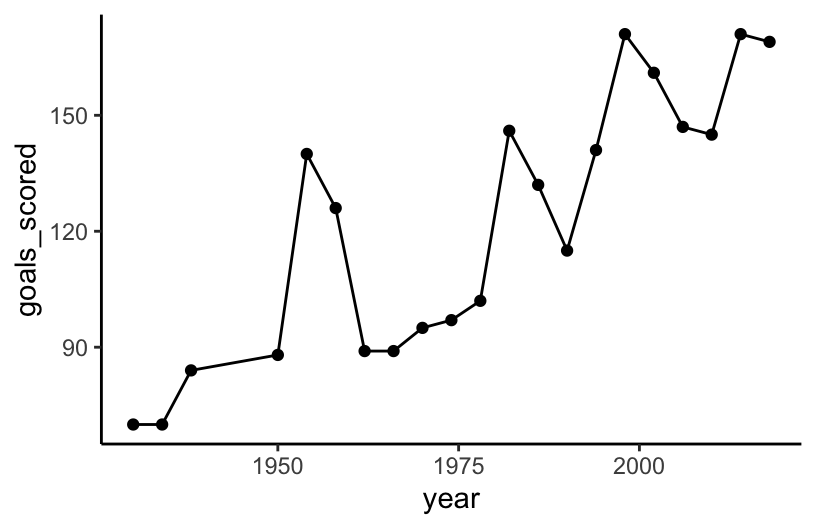

# Our above summaries might be a bit misleading.
# The number of games played at the World Cup varies.
# Construct a bivariate plot of how the typical number of goals per game has changed over the years
per_game_data <- world_cup %>% 
  mutate(goals_per_game = goals_scored / games)

ggplot(per_game_data, aes(x = year, y = goals_per_game)) + 
  geom_point() + 
  geom_line()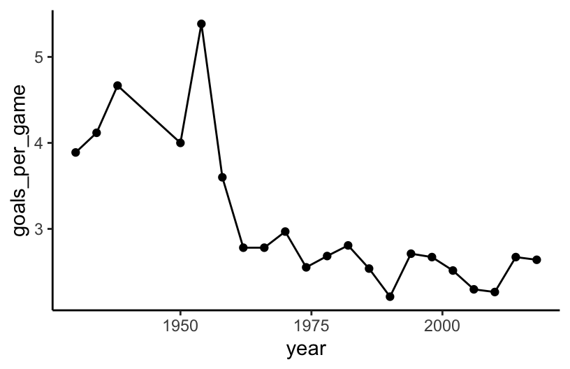

Exercise 11: More viz review

mn_wi_new <- elections %>%
  filter(state_name %in% c("Minnesota", "Wisconsin")) %>%
  mutate(repub_win_20 = (repub_pct_20 > dem_pct_20),
          repub_win_16 = (repub_pct_16 > dem_pct_16),
          ) %>%
  select(state_abbr, repub_pct_20, repub_pct_16, repub_pct_12, repub_win_20, repub_win_16)
head(mn_wi_new)
##   state_abbr repub_pct_20 repub_pct_16 repub_pct_12 repub_win_20 repub_win_16
## 1         MN        62.42        60.05        49.76         TRUE         TRUE
## 2         MN        49.69        50.71        50.31         TRUE         TRUE
## 3         MN        64.11        63.66        56.37         TRUE         TRUE
## 4         MN        50.39        50.59        43.91         TRUE         TRUE
## 5         MN        64.61        64.65        55.58         TRUE         TRUE
## 6         MN        62.64        58.89        49.77         TRUE         TRUE

# Construct a plot that illustrates the relationship of  repub_pct_20 with repub_pct_16 and repub_pct_12
ggplot(mn_wi_new, aes(y = repub_pct_20, x = repub_pct_16, color = repub_pct_12)) +
  geom_point()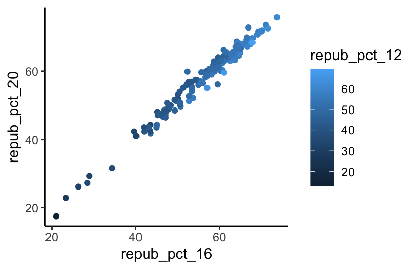

# Construct a plot that illustrates the relationship of  repub_pct_20 with repub_pct_16 in MN vs WI.
# Do this in 1 frame and add a linear trend
ggplot(mn_wi_new, aes(y = repub_pct_20, x = repub_pct_16, color = state_abbr)) +
  geom_point() +
  geom_smooth(method = "lm")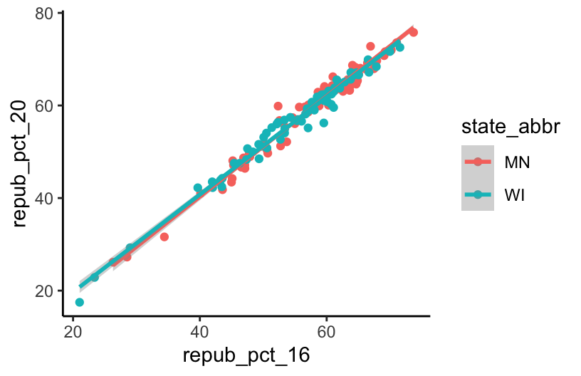

# Construct a plot that illustrates the relationship of  repub_pct_20 with repub_pct_16 in MN vs WI.
# Do this in 2 separate frames -- 1 for MN and 1 for WI
# and include linear trends
ggplot(mn_wi_new, aes(y = repub_pct_20, x = repub_pct_16, color = state_abbr)) +
  geom_point() +
  geom_smooth(method = "lm") +
  facet_wrap(~ state_abbr)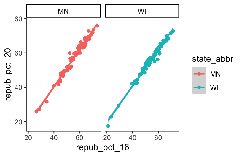

# Construct a plot that illustrates how many counties were
# won by the republican in 2020, combining MN and WI counties
ggplot(mn_wi_new, aes(x = repub_win_20)) +
  geom_bar()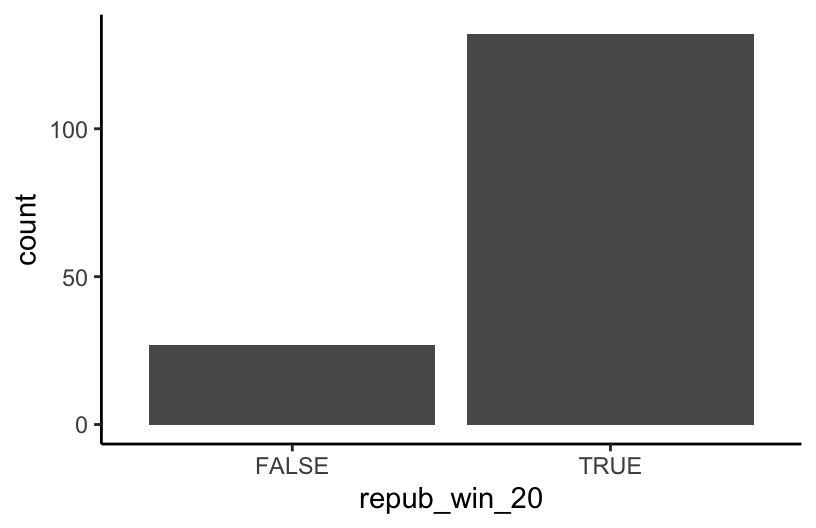

# Construct a plot that illustrates how many counties were
# won by the republican in 2020 in MN vs WI, i.e.
# the relationship between `state_abbr` and `repub_win_20`
ggplot(mn_wi_new, aes(x = state_abbr, fill = repub_win_20)) +
  geom_bar()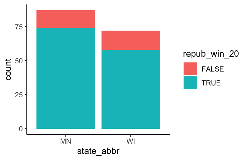

# Starting with the previous plot, and if you didn't already,
# tweak it so that we can directly compare the proportion
# of counties won by the republican in 2020 in MN and WI,
# ignoring the fact that MN has more counties
ggplot(mn_wi_new, aes(x = state_abbr, fill = repub_win_20)) +
  geom_bar(position = "fill")

8.1 Data wrangling motivation

8.2 Warm-up

8.3 Exercises

Exercise 1: select practice

Exercise 2: filter demo

Exercise 3: arrange demo

Exercise 4: mutate demo

Part a

Part b

Exercise 5: Pipe series

Part a

Part b

Part c

Part d

Part e

Exercise 6: DIY pipe series

Part a

Part b

Part c

Exercise 7: summarize demo

Exercise 8: summarize + group_by demo

Exercise 9: DIY

Part a

Part b

Exercise 10: Practice on new data

Exercise 11: More viz review

8.4 Wrap-up

8.5 Solutions

8.5.1 EXAMPLE 1

Exercise 1: select practice

Exercise 2: filter demo

Exercise 3: arrange demo

Exercise 4: mutate demo

Exercise 5: Pipe series

Part c

Part e

Exercise 6: DIY pipe series

Part a

Part b

Part c

Exercise 7: summarize demo

Exercise 8: summarize + group_by demo

Exercise 9: DIY

Part a

Exercise 10: Practice on new data

Exercise 11: More viz review

Exercise 8: `summarize` + `group_by` demo

Exercise 8: `summarize` + `group_by` demo