library(tidyverse)
penguins <- read_csv('https://raw.githubusercontent.com/rfordatascience/tidytuesday/master/data/2020/2020-07-28/penguins.csv')

# Check it out
head(penguins)
## # A tibble: 6 × 8
##   species island    bill_length_mm bill_depth_mm flipper_length_mm body_mass_g
##   <chr>   <chr>              <dbl>         <dbl>             <dbl>       <dbl>
## 1 Adelie  Torgersen           39.1          18.7               181        3750
## 2 Adelie  Torgersen           39.5          17.4               186        3800
## 3 Adelie  Torgersen           40.3          18                 195        3250
## 4 Adelie  Torgersen           NA            NA                  NA          NA
## 5 Adelie  Torgersen           36.7          19.3               193        3450
## 6 Adelie  Torgersen           39.3          20.6               190        3650
## # ℹ 2 more variables: sex <chr>, year <dbl>9 Wrangling practice
Learning goals
- Practice using the following wrangling verbs appropriately:
select,mutate,filter,arrange,summarize,group_by - Start to develop an understanding what code will do conceptually without running it
- Start to develop a knowledge of working with dates and
lubridatefunctions
Additional resources
Quick Review
Alternative Text
Guide for Alt Text for Data Viz
Washington Post’s Alt Text Guidelines
Alt text should concisely articulate:
- What your visualization is (e.g. a density plot of 3pm temperatures in Hobart, Uluru, and Wollongong, Australia).
- What your visualization looks like aka the visual elements themselves (e.g. describe how the 3 density curves and the plotting frame appear).
- A 1-sentence description of the most important takeaway.
- A link or description of your data source if it’s not already in the caption.
For Quiz 1, I’m not “grading” the alt text problem. I’d like everyone to try it again.
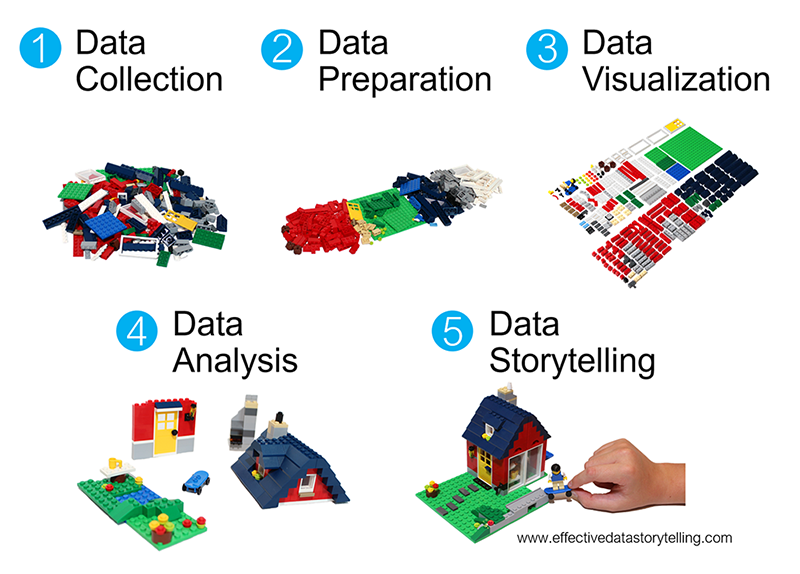
Where are we? Data preparation
Reminder
You will make mistakes.
Mistakes are important to learning. AND You will always make mistakes – you will just get better at fixing mistakes and avoiding the most common mistakes.
9.1 Warm-up
RECALL
Wrangling is important :). It’s much of what we spend our efforts on in Data Science. There are lots of steps, hence R functions, that can go into data wrangling. But we can get far with the following 6 wrangling verbs:
| verb | action |
|---|---|
arrange |
arrange the rows according to some column |
filter |
filter out or obtain a subset of the rows |
select |
select a subset of columns |
mutate |
mutate or create a column |
summarize |
calculate a numerical summary of a column |
group_by |
group the rows by a specified column |

EXAMPLE 1: Viz practice
Let’s start by working with some TidyTuesday data on penguins. This data includes information about penguins’ flippers (“arms”) and bills (“mouths” or “beaks”). Image source.

Let’s import this using read_csv(), a function in the tidyverse package. For the most part, this is similar to read.csv(), though read_csv() can be more efficient at importing large datasets.
Construct a plot that allows us to examine how the relationship between body mass and bill length varies by species and sex.
EXAMPLE 2: verb review
Use the 6 wrangling verbs to address each task below. You can tack on %>% head() to print out just 6 rows to keep your rendered document manageable. Most of these require just 1 verb.
# Get data on only Adelie penguins that weigh more than 4700g


# Get data on penguin body mass only
# Show just the first 6 rows


# Sort the penguins from smallest to largest body mass
# Show just the first 6 rows


# Calculate the average body mass across all penguins
# Note: na.rm = TRUE removes the NAs from the calculation


# Calculate the average body mass by species


# Create a new column that records body mass in kilograms, not grams
# NOTE: there are 1000 g in 1 kg
# Show just the first 6 rows
EXAMPLE 3: Counting
How many penguins of each species do we have? Create a viz that addresses this question.
ggplot(penguins, aes(x = species))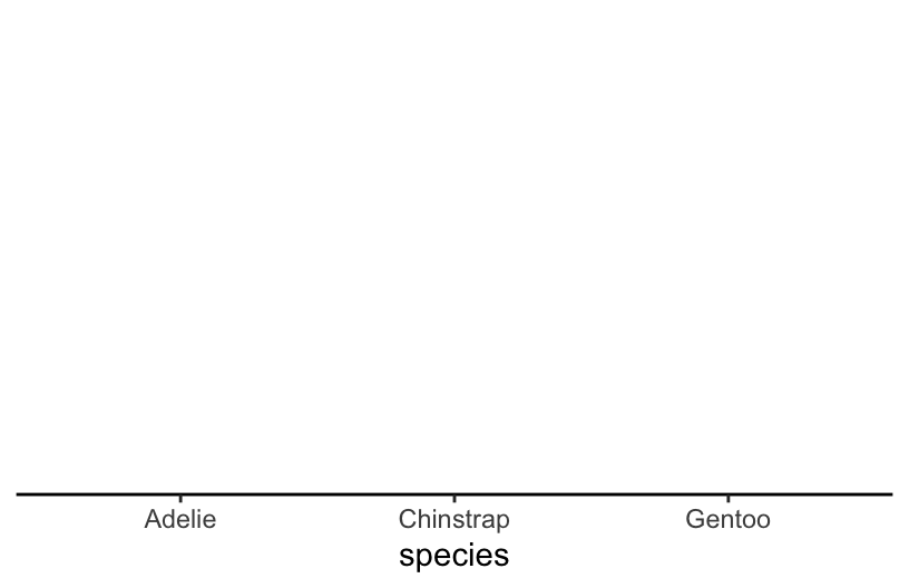
To be more precise, we can calculate the number of penguins of each species using our 6 verbs. HINT: n() calculates group size.
The count() verb provides a handy shortcut to the group_by() %>% summarize() for counting!
penguins %>%
  count(species)
## # A tibble: 3 × 2
##   species       n
##   <chr>     <int>
## 1 Adelie      152
## 2 Chinstrap    68
## 3 Gentoo      124
EXAMPLE 4: Multiple verbs
Let’s practice combining some verbs. For each task:
- Translate the prompt into our 6 verbs. That is, think before you type.
- Build your code line by line. It’s important to understand what’s being piped into each function!
- Ask what you can rearrange and still get the same result.
- Read your final code like a paragraph / a conversation. Would another person be able to follow your logic?
# Sort Gentoo penguins from biggest to smallest with respect to their
# bill length in cm (there are 10 mm in a cm)
# Sort the species from smallest to biggest with respect to their
# average bill length in cm
EXAMPLE 5: Interpret this code
Let’s practice reading and making sense of somebody else’s code. What do you think this produces?
- How many columns? Rows?
- What are the column names?
- What’s represented in each row?
Once you’ve thought about it, put the code inside a chunk and run it!
penguins %>% filter(species == “Chinstrap”) %>% group_by(sex) %>% summarize(min = min(body_mass_g), max = max(body_mass_g)) %>% mutate(range = max - min)
9.2 Exercises Part 1: Same verbs, new tricks
Goals
- Part 1
- Learn some new ways to use our 6 verbs, using the penguins.
- Explore how to work dates (eg: “2024-02-20”).
- Part 2: You will practice wrangling using the birthday data you explored visually in Homework 1. These are similar to exercises that will be on Homework 4.
Directions
- Work together!
- Stay on track / focused on this activity. This is helpful to you, and the students around you :)
Exercise 1: More filtering
Recall the “logical comparison operators” we can use to filter() our data:
| symbol | meaning |
|---|---|
| == | equal to |
| != | not equal to |
| > | greater than |
| >= | greater than or equal to |
| < | less than |
| <= | less than or equal to |
| %in% c(, ) | a list of multiple values |
Part a
# Create a dataset with just Adelie and Chinstrap using %in%
# Pipe this into `count(species)` to confirm that you only have these 2 species
# ___ %>%
# filter(___) %>%
# count(species)# Create a dataset with just Adelie and Chinstrap using !=
# Pipe this into `count(species)` to confirm that you only have these 2 species
# ___ %>%
# filter(___) %>%
# count(species)Part b
Notice that some of our penguins have missing (NA) data on some values:
head(penguins)
## # A tibble: 6 × 8
## species island bill_length_mm bill_depth_mm flipper_length_mm body_mass_g
## <chr> <chr> <dbl> <dbl> <dbl> <dbl>
## 1 Adelie Torgersen 39.1 18.7 181 3750
## 2 Adelie Torgersen 39.5 17.4 186 3800
## 3 Adelie Torgersen 40.3 18 195 3250
## 4 Adelie Torgersen NA NA NA NA
## 5 Adelie Torgersen 36.7 19.3 193 3450
## 6 Adelie Torgersen 39.3 20.6 190 3650
## # ℹ 2 more variables: sex <chr>, year <dbl>There are many ways to handle this. The right approach depends upon your research goals. A general rule is: Only get rid of observations with missing data if they’re missing data on variables you need for the specific task at hand!
Example 1
Suppose our research focus is just on body_mass_g. 2 penguins are missing this info:
# NOTE the use of is.na()
penguins %>%
summarize(sum(is.na(body_mass_g)))
## # A tibble: 1 × 1
## `sum(is.na(body_mass_g))`
## <int>
## 1 2Let’s define a new dataset that removes these penguins:
# NOTE the use of is.na()
penguins_w_body_mass <- penguins %>%
filter(!is.na(body_mass_g))
# Compare the number of penguins in this vs the original data
nrow(penguins_w_body_mass)
## [1] 342
nrow(penguins)
## [1] 344Note that some penguins in penguins_w_body_mass are missing info on sex, but we don’t care since that’s not related to our research question:
penguins_w_body_mass %>%
summarize(sum(is.na(sex)))
## # A tibble: 1 × 1
## `sum(is.na(sex))`
## <int>
## 1 9Example 2
In the very rare case that we need complete information on every variable for the specific task at hand, we can use na.omit() to get rid of any penguin that’s missing info on any variable:
penguins_complete <- penguins %>%
na.omit()How many penguins did this eliminate?
nrow(penguins_complete)
## [1] 333
nrow(penguins)
## [1] 344Part c
Explain why we should only use na.omit() in extreme circumstances.
Exercise 2: More selecting
Being able to select() only certain columns can help simplify our data. This is especially important when we’re working with lots of columns (which we haven’t done yet). It can also get tedious to type out every column of interest. Here are some shortcuts:
-removes a given variable and keeps all others (e.g.select(-island))starts_with("___"),ends_with("___"), orcontains("___")selects only the columns that either start with, end with, or simply contain the given string of characters
Use these shortcuts to create the following datasets.
# First: recall the variable names
names(penguins)
## [1] "species" "island" "bill_length_mm"
## [4] "bill_depth_mm" "flipper_length_mm" "body_mass_g"
## [7] "sex" "year"# Use a shortcut to keep everything but the year and island variables# Use a shortcut to keep only species and the penguin characteristics measured in mm# Use a shortcut to keep only species and bill-related measurements# Use a shortcut to keep only species and the length-related characteristics
Exercise 3: Arranging, counting, & grouping by multiple variables
We’ve done examples where we need to filter() by more than one variable, or select() more than one variable. Use your intuition for how we can arrange(), count(), and group_by() more than one variable.
# Change this code to sort the penguins by species, and then island name
# NOTE: The first row should be an Adelie penguin living on Biscoe island
penguins %>%
arrange(species)
## # A tibble: 344 × 8
## species island bill_length_mm bill_depth_mm flipper_length_mm body_mass_g
## <chr> <chr> <dbl> <dbl> <dbl> <dbl>
## 1 Adelie Torgersen 39.1 18.7 181 3750
## 2 Adelie Torgersen 39.5 17.4 186 3800
## 3 Adelie Torgersen 40.3 18 195 3250
## 4 Adelie Torgersen NA NA NA NA
## 5 Adelie Torgersen 36.7 19.3 193 3450
## 6 Adelie Torgersen 39.3 20.6 190 3650
## 7 Adelie Torgersen 38.9 17.8 181 3625
## 8 Adelie Torgersen 39.2 19.6 195 4675
## 9 Adelie Torgersen 34.1 18.1 193 3475
## 10 Adelie Torgersen 42 20.2 190 4250
## # ℹ 334 more rows
## # ℹ 2 more variables: sex <chr>, year <dbl># Change this code to count the number of male/female penguins observed for each species
penguins %>%
count(species)
## # A tibble: 3 × 2
## species n
## <chr> <int>
## 1 Adelie 152
## 2 Chinstrap 68
## 3 Gentoo 124# Change this code to calculate the average body mass by species and sex
penguins %>%
group_by(species) %>%
summarize(mean = mean(body_mass_g, na.rm = TRUE))
## # A tibble: 3 × 2
## species mean
## <chr> <dbl>
## 1 Adelie 3701.
## 2 Chinstrap 3733.
## 3 Gentoo 5076.
Exercise 4: Dates
Before some wrangling practice, let’s explore another important concept: working with or mutating date variables. Dates are a whole special object type or class in RStudio that automatically respect the order of time.
# Get today's date
as.Date(today())
## [1] "2024-12-03"
# Let's store this as "today" so we can work with it below
today <- as.Date(today())
# Check out the class of this object
class(today)
## [1] "Date"The lubridate package inside tidyverse contains functions that can extract various information from dates. Let’s learn about some of the most common functions by applying them to today. For each, make a comment on what the function does
year(today)
## [1] 2024# What do these lines produce / what's their difference?
month(today)
## [1] 12
month(today, label = TRUE)
## [1] Dec
## 12 Levels: Jan < Feb < Mar < Apr < May < Jun < Jul < Aug < Sep < ... < Dec# What does this number mean?
week(today)
## [1] 49# What do these lines produce / what's their difference?
mday(today)
## [1] 3
yday(today) # This is often called the "Julian day"
## [1] 338# What do these lines produce / what's their difference?
wday(today)
## [1] 3
wday(today, label = TRUE)
## [1] Tue
## Levels: Sun < Mon < Tue < Wed < Thu < Fri < Sat# What do the results of these 2 lines tell us?
today >= ymd("2024-02-14")
## [1] TRUE
today < ymd("2024-02-14")
## [1] FALSE
9.3 Exercises Part 2: Application
RECALL: The remaining exercises are similar to some on Homework 4, thus solutions aren’t provided.
Let’s apply these ideas to the daily Birthdays dataset in the mosaic package that we explored in Homework 2:
library(mosaic)
data("Birthdays")
head(Birthdays)
## state year month day date wday births
## 1 AK 1969 1 1 1969-01-01 Wed 14
## 2 AL 1969 1 1 1969-01-01 Wed 174
## 3 AR 1969 1 1 1969-01-01 Wed 78
## 4 AZ 1969 1 1 1969-01-01 Wed 84
## 5 CA 1969 1 1 1969-01-01 Wed 824
## 6 CO 1969 1 1 1969-01-01 Wed 100Birthdays gives the number of births recorded on each day of the year in each state from 1969 to 1988.1 We can use our wrangling skills to understand some drivers of daily births. Putting these all together can be challenging! Remember the following ways to make tasks more manageable:
- Translate the prompt into our 6 verbs (and
count()). That is, think before you type. - Build your code line by line. It’s important to understand what’s being piped into each function!
Exercise 5: Warming up
# How many days of data do we have for each state?
# How many total births were there in this time period?
# How many total births were there per state in this time period, sorted from low to high?
Exercise 6: Homework 2 reprise
Create a new dataset named daily_births that includes the total number of births per day (across all states) and the corresponding day of the week (eg: Mon). NOTE: Name the column with total births so that it’s easier to wrangle and plot.
Using this data, construct a plot of births over time, indicating the day of week.
Exercise 7: Wrangle & plot
For each prompt below, you can decide whether you want to: (1) wrangle and store data, then plot; or (2) wrangle data and pipe directly into ggplot. For example:
penguins %>%
filter(species != "Gentoo") %>%
ggplot(aes(y = bill_length_mm, x = bill_depth_mm, color = species)) +
geom_point()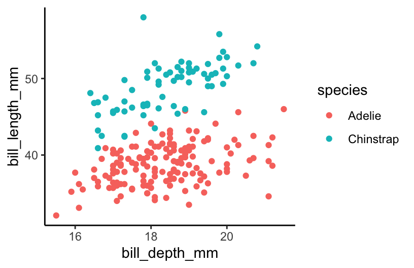
Part a
Calculate the total number of births in each month and year (eg: Jan 1969, Feb 1969, …). Label month by names not numbers (Jan not 1). Then plot the births by month and comment on what you learn.
Part b
In 1988, calculate the total number of births per week in each state. (Get rid of week “53”, which isn’t a complete week!) Then make a line plot of births by week for each state, and comment on what you learn. For example, do you notice any seasonal trends? Are these the same in every state? Any outliers?
Part c
Repeat the above for just Minnesota (MN) and Louisiana (LA). MN has one of the coldest climates, and LA has one of the warmest. How do their seasonal trends compare? (Do you think these trends are similar in other colder and warmer states? Try it!)
Exercise 8: More practice
Part a
Create a dataset with only births in Massachusetts (MA) in 1979, and sort the days from those with the most births to those with the fewest.
Part b
Make a table showing the five states with the most births between September 9, 1979 and September 12, 1979, including the 9th and 12th. Arrange the table in descending order of births.
9.4 Wrap-up
- Make sure to complete the checkpoint before the next class.
- Review the exercises after class that you didn’t get to today.
- Start Homework 4.
9.5 Solutions
Click for Solutions
EXAMPLE 1: Viz practice
ggplot(penguins, aes(y = body_mass_g, x = bill_length_mm, color = species)) +
geom_point() +
facet_wrap(~ sex)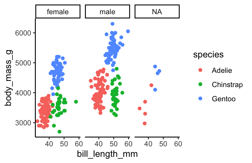
EXAMPLE 2: verb review
# Get data on only Adelie penguins that weigh more than 4700g
penguins %>%
filter(species == "Adelie", body_mass_g > 4700)
## # A tibble: 2 × 8
## species island bill_length_mm bill_depth_mm flipper_length_mm body_mass_g
## <chr> <chr> <dbl> <dbl> <dbl> <dbl>
## 1 Adelie Biscoe 41 20 203 4725
## 2 Adelie Biscoe 43.2 19 197 4775
## # ℹ 2 more variables: sex <chr>, year <dbl>
# Get data on penguin body mass only
# Show just the first 6 rows
penguins %>%
select(body_mass_g) %>%
head()
## # A tibble: 6 × 1
## body_mass_g
## <dbl>
## 1 3750
## 2 3800
## 3 3250
## 4 NA
## 5 3450
## 6 3650
# Sort the penguins from smallest to largest body mass
# Show just the first 6 rows
penguins %>%
arrange(body_mass_g) %>%
head()
## # A tibble: 6 × 8
## species island bill_length_mm bill_depth_mm flipper_length_mm body_mass_g
## <chr> <chr> <dbl> <dbl> <dbl> <dbl>
## 1 Chinstrap Dream 46.9 16.6 192 2700
## 2 Adelie Biscoe 36.5 16.6 181 2850
## 3 Adelie Biscoe 36.4 17.1 184 2850
## 4 Adelie Biscoe 34.5 18.1 187 2900
## 5 Adelie Dream 33.1 16.1 178 2900
## 6 Adelie Torgersen 38.6 17 188 2900
## # ℹ 2 more variables: sex <chr>, year <dbl>
# Calculate the average body mass across all penguins
# Note: na.rm = TRUE removes the NAs from the calculation
penguins %>%
summarize(mean = mean(body_mass_g, na.rm = TRUE))
## # A tibble: 1 × 1
## mean
## <dbl>
## 1 4202.
# Calculate the average body mass by species
penguins %>%
group_by(species) %>%
summarize(mean = mean(body_mass_g, na.rm = TRUE))
## # A tibble: 3 × 2
## species mean
## <chr> <dbl>
## 1 Adelie 3701.
## 2 Chinstrap 3733.
## 3 Gentoo 5076.
# Create a new column that records body mass in kilograms, not grams
# NOTE: there are 1000 g in 1 kg
# Show just the first 6 rows
penguins %>%
mutate(body_mass_kg = body_mass_g/1000) %>%
head()
## # A tibble: 6 × 9
## species island bill_length_mm bill_depth_mm flipper_length_mm body_mass_g
## <chr> <chr> <dbl> <dbl> <dbl> <dbl>
## 1 Adelie Torgersen 39.1 18.7 181 3750
## 2 Adelie Torgersen 39.5 17.4 186 3800
## 3 Adelie Torgersen 40.3 18 195 3250
## 4 Adelie Torgersen NA NA NA NA
## 5 Adelie Torgersen 36.7 19.3 193 3450
## 6 Adelie Torgersen 39.3 20.6 190 3650
## # ℹ 3 more variables: sex <chr>, year <dbl>, body_mass_kg <dbl>
EXAMPLE 3: Counting
ggplot(penguins, aes(x = species)) +
geom_bar()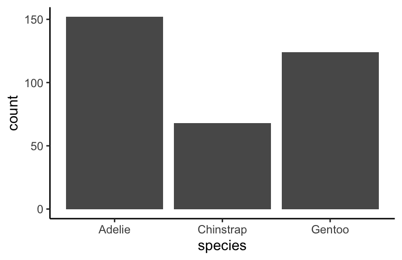
penguins %>%
group_by(species) %>%
summarize(n())
## # A tibble: 3 × 2
## species `n()`
## <chr> <int>
## 1 Adelie 152
## 2 Chinstrap 68
## 3 Gentoo 124
penguins %>%
count(species)
## # A tibble: 3 × 2
## species n
## <chr> <int>
## 1 Adelie 152
## 2 Chinstrap 68
## 3 Gentoo 124
EXAMPLE 4: Multiple verbs
# Sort Gentoo penguins from biggest to smallest with respect to their
# bill length in cm (there are 10 mm in a cm)
penguins %>%
filter(species == "Gentoo") %>%
mutate(bill_length_cm = bill_length_mm / 10) %>%
arrange(desc(bill_length_cm))
## # A tibble: 124 × 9
## species island bill_length_mm bill_depth_mm flipper_length_mm body_mass_g
## <chr> <chr> <dbl> <dbl> <dbl> <dbl>
## 1 Gentoo Biscoe 59.6 17 230 6050
## 2 Gentoo Biscoe 55.9 17 228 5600
## 3 Gentoo Biscoe 55.1 16 230 5850
## 4 Gentoo Biscoe 54.3 15.7 231 5650
## 5 Gentoo Biscoe 53.4 15.8 219 5500
## 6 Gentoo Biscoe 52.5 15.6 221 5450
## 7 Gentoo Biscoe 52.2 17.1 228 5400
## 8 Gentoo Biscoe 52.1 17 230 5550
## 9 Gentoo Biscoe 51.5 16.3 230 5500
## 10 Gentoo Biscoe 51.3 14.2 218 5300
## # ℹ 114 more rows
## # ℹ 3 more variables: sex <chr>, year <dbl>, bill_length_cm <dbl>
# Sort the species from smallest to biggest with respect to their
# average bill length in cm
penguins %>%
mutate(bill_length_cm = bill_length_mm / 10) %>%
group_by(species) %>%
summarize(mean_bill_length = mean(bill_length_cm, na.rm = TRUE)) %>%
arrange(desc(mean_bill_length))
## # A tibble: 3 × 2
## species mean_bill_length
## <chr> <dbl>
## 1 Chinstrap 4.88
## 2 Gentoo 4.75
## 3 Adelie 3.88
EXAMPLE 5: Interpret this code
Exercise 1: More filtering
Part a
# Create a dataset with just Adelie and Chinstrap using %in%
# Pipe this into `count(species)` to confirm that you only have these 2 species
penguins %>%
filter(species %in% c("Adelie", "Chinstrap")) %>%
count(species)
## # A tibble: 2 × 2
## species n
## <chr> <int>
## 1 Adelie 152
## 2 Chinstrap 68# Create a dataset with just Adelie and Chinstrap using !=
# Pipe this into `count(species)` to confirm that you only have these 2 species
penguins %>%
filter(species != "Gentoo") %>%
count(species)
## # A tibble: 2 × 2
## species n
## <chr> <int>
## 1 Adelie 152
## 2 Chinstrap 68Part b
Part c
It might get rid of data points even if they have complete information on the variables we need, just because they’re missing info on variables we don’t need.
Exercise 2: More selecting
# First: recall the variable names
names(penguins)
## [1] "species"           "island"            "bill_length_mm"
## [4] "bill_depth_mm"     "flipper_length_mm" "body_mass_g"
## [7] "sex"               "year"
# Use a shortcut to keep everything but the year and island variables
penguins %>%
select(-year, -island)
## # A tibble: 344 × 6
## species bill_length_mm bill_depth_mm flipper_length_mm body_mass_g sex
## <chr> <dbl> <dbl> <dbl> <dbl> <chr>
## 1 Adelie 39.1 18.7 181 3750 male
## 2 Adelie 39.5 17.4 186 3800 female
## 3 Adelie 40.3 18 195 3250 female
## 4 Adelie NA NA NA NA <NA>
## 5 Adelie 36.7 19.3 193 3450 female
## 6 Adelie 39.3 20.6 190 3650 male
## 7 Adelie 38.9 17.8 181 3625 female
## 8 Adelie 39.2 19.6 195 4675 male
## 9 Adelie 34.1 18.1 193 3475 <NA>
## 10 Adelie 42 20.2 190 4250 <NA>
## # ℹ 334 more rows# Use a shortcut to keep only species and the penguin characteristics measured in mm
penguins %>%
select(species, ends_with("mm"))
## # A tibble: 344 × 4
## species bill_length_mm bill_depth_mm flipper_length_mm
## <chr> <dbl> <dbl> <dbl>
## 1 Adelie 39.1 18.7 181
## 2 Adelie 39.5 17.4 186
## 3 Adelie 40.3 18 195
## 4 Adelie NA NA NA
## 5 Adelie 36.7 19.3 193
## 6 Adelie 39.3 20.6 190
## 7 Adelie 38.9 17.8 181
## 8 Adelie 39.2 19.6 195
## 9 Adelie 34.1 18.1 193
## 10 Adelie 42 20.2 190
## # ℹ 334 more rows# Use a shortcut to keep only species and bill-related measurements
penguins %>%
select(species, starts_with("bill"))
## # A tibble: 344 × 3
## species bill_length_mm bill_depth_mm
## <chr> <dbl> <dbl>
## 1 Adelie 39.1 18.7
## 2 Adelie 39.5 17.4
## 3 Adelie 40.3 18
## 4 Adelie NA NA
## 5 Adelie 36.7 19.3
## 6 Adelie 39.3 20.6
## 7 Adelie 38.9 17.8
## 8 Adelie 39.2 19.6
## 9 Adelie 34.1 18.1
## 10 Adelie 42 20.2
## # ℹ 334 more rows# Use a shortcut to keep only species and the length-related characteristics
penguins %>%
select(species, contains("length"))
## # A tibble: 344 × 3
## species bill_length_mm flipper_length_mm
## <chr> <dbl> <dbl>
## 1 Adelie 39.1 181
## 2 Adelie 39.5 186
## 3 Adelie 40.3 195
## 4 Adelie NA NA
## 5 Adelie 36.7 193
## 6 Adelie 39.3 190
## 7 Adelie 38.9 181
## 8 Adelie 39.2 195
## 9 Adelie 34.1 193
## 10 Adelie 42 190
## # ℹ 334 more rows
Exercise 3: Arranging, counting, & grouping by multiple variables
# Change this code to sort the penguins by species, and then island name
# NOTE: The first row should be an Adelie penguin living on Biscoe island
penguins %>%
arrange(species, island) %>%
head()
## # A tibble: 6 × 8
## species island bill_length_mm bill_depth_mm flipper_length_mm body_mass_g
## <chr> <chr> <dbl> <dbl> <dbl> <dbl>
## 1 Adelie Biscoe 37.8 18.3 174 3400
## 2 Adelie Biscoe 37.7 18.7 180 3600
## 3 Adelie Biscoe 35.9 19.2 189 3800
## 4 Adelie Biscoe 38.2 18.1 185 3950
## 5 Adelie Biscoe 38.8 17.2 180 3800
## 6 Adelie Biscoe 35.3 18.9 187 3800
## # ℹ 2 more variables: sex <chr>, year <dbl># Change this code to count the number of male/female penguins observed for each species
penguins %>%
count(species, sex)
## # A tibble: 8 × 3
## species sex n
## <chr> <chr> <int>
## 1 Adelie female 73
## 2 Adelie male 73
## 3 Adelie <NA> 6
## 4 Chinstrap female 34
## 5 Chinstrap male 34
## 6 Gentoo female 58
## 7 Gentoo male 61
## 8 Gentoo <NA> 5# Change this code to calculate the average body mass by species and sex
penguins %>%
group_by(species, sex) %>%
summarize(mean = mean(body_mass_g, na.rm = TRUE))
## # A tibble: 8 × 3
## # Groups: species [3]
## species sex mean
## <chr> <chr> <dbl>
## 1 Adelie female 3369.
## 2 Adelie male 4043.
## 3 Adelie <NA> 3540
## 4 Chinstrap female 3527.
## 5 Chinstrap male 3939.
## 6 Gentoo female 4680.
## 7 Gentoo male 5485.
## 8 Gentoo <NA> 4588.
Exercise 4: Dates
# Get today's date
as.Date(today())
## [1] "2024-12-03"

# Let's store this as "today" so we can work with it below
today <- as.Date(today())

# Check out the class of this object
class(today)
## [1] "Date"# Records just the 4-digit year
year(today)
## [1] 2024
# Today's month, as a number or label
month(today)
## [1] 12
month(today, label = TRUE)
## [1] Dec
## 12 Levels: Jan < Feb < Mar < Apr < May < Jun < Jul < Aug < Sep < ... < Dec# This is the week of the year (1-52)
week(today)
## [1] 49# Day of the month (1-31) and day of the year (1-366)
mday(today)
## [1] 3
yday(today) # This is often called the "Julian day"
## [1] 338# Day of the week as a number or label
wday(today)
## [1] 3
wday(today, label = TRUE)
## [1] Tue
## Levels: Sun < Mon < Tue < Wed < Thu < Fri < Sat# today is on or after Feb 14, 2024
today >= ymd("2024-02-14")
## [1] TRUE
# today is not before Feb 14, 2024
today < ymd("2024-02-14")
## [1] FALSE
The
fivethirtyeightpackage has more recent data.↩︎