7.2 Point Processes

A point pattern/process data set gives the locations of objects/events occuring in a study region. These points could represent trees, animal nests, earthquake epicenters, crimes, cases of influenza, galaxes, etc. We are assuming that the occurance or non occurance of a point at a location is random.

The observed points may have extra information called marks attached to them. These marks represent an attribute or characteristic of the point. These could be categorical or continuous.

7.2.1 Poisson Point Processes

The underlying probability model we assume determes the number of occurances of events in a small area is going to be a Poisson model with parameter \(\lambda(s)\), the intensity in a fixed area. This intensity may be constant (uniform) across locations or may vary from location to location (inhomogeneous).

For a homogenous Poisson process, we model the number of points in any region \(A\), \(N(A)\), to be Poisson with

\[E(N(A)) = \lambda\cdot\text{Area}(A)\]

such that \(\lambda\) is constant across space. Given \(N(A) = n\), the \(N\) events form an iid sample from the uniform distribution on \(A\). Under this model, for any two disjoint regions \(A\) and \(B\), the random variables \(N(A)\) and \(N(B)\) are independent.

If we observe \(n\) events in region \(A\), the estimator \(\hat{\lambda} = n/\text{Area(A)}\) is unbiased, if the model is correct.

This homogenous Poisson model is also known as complete spatial randomness (CSR). If points deviate from it, we might be able to detect this with a hypothesis test. We’ll come back to this when we discuss distances to neighbors.

To simulate data from a CSR process in a square [0,1]x[0,1], we could

Generate the number of events from a Poisson distribution with \(\lambda\)

n <- rpois(1, lambda = 50)

Fix n and generate locations from the uniform

x <- runif(n, 0, 1)
y <- runif(n, 0, 1)
plot(x, y)

Alternatively, have generate the data with rpoispp.

sim1 <- rpoispp(lambda = 50)
plot(sim1)

If the intensity is not constant across space (inhomogenous Poisson process), then we define intensity as

\[\lambda(s) = \lim_{|ds|\rightarrow 0} \frac{E(N(ds))}{|ds|}\]

where \(ds\) is a small area element and \(N(A)\) has a Poisson distribution with mean

\[\mu(A) = \int_A \lambda(s)ds\]

When working with point process data, we generally will want to estimate and/or model \(\lambda(s)\) in a region \(A\) and determine if \(\lambda(s) = \lambda\) for \(s\in A\).

7.2.2 Non-Parametric Intensity Estimation

7.2.2.1 Quadrat Estimation

One way to estimate the intensity \(\lambda(s)\) requires that the study area be divided into sub-regions (also known as quadrats). Then, the estimated density is computed for each quadrat by dividing the number of points in each quadrat by the quadrat’s area. Quadrats can take on many different shapes such as hexagons and triangles or the typically square-shaped quadrats.

If the points have uniform/constant intensity (CSR), then the quadrat counts should be Poisson random numbers with constant mean. Using a \(\chi^2\) goodness-of-fit test statistic, we can test \(H_0:\) CSR,

plot(quadratcount(bei, nx = 4, ny = 4))

(T <- quadrat.test(bei, nx = 4, ny = 4))

## 
##  Chi-squared test of CSR using quadrat counts
## 
## data:  bei
## X2 = 1755, df = 15, p-value <2e-16
## alternative hypothesis: two.sided
## 
## Quadrats: 4 by 4 grid of tiles

plot(bei)
plot(T, add = TRUE)

The choice of quadrat numbers and quadrat shape can influence the estimated density and must be chosen with care. If the quadrats are too small, you risk having many quadrats with no points which may prove uninformative (and can cause issues if you are trying to run a \(\chi^2\) test). If very large quadrat sizes are used, you risk missing subtle changes in spatial density.

If the density is not uniform across the space, you should wonder why. Is there a covariate (characteristic of the space that could be collected at every point in space) that could help explain the difference in the intensity? For example, perhaps the elevation of an area could be impacting the intensity of trees that thrive in the area. Or there could be a west/east or north/south pattern such that the longitude or latitude impacts the intensity.

If there is a covariate, we can convert the covariate across the continuous spatial field into discretized areas. We can then plot the relationship between the estimated point density within the quadrat and the covariate regions to assess any dependence between variables. If there is a clear relationship, the levels of the covariate can define new sub-regions within which the density can be computed. This is the idea of normalizing data by some underlying covariate.

The quadrat analysis approach has its advantages in that it is easy to compute and interpret; however, it does suffer from the modifiable areal unit problem (MAUP) as the relationship observed can change depending on the size and shape of the quadrats chosen. Another density based approach that will be explored next (and that is less susceptible to the MAUP) is the kernel density estimation process.

7.2.2.2 Kernel Density Estimation

The kernel density approach is an extension of the quadrat method. Like the quadrat density, the kernel approach computes a localized density for subsets of the study area, but unlike its quadrat density counterpart, the sub-regions overlap one another providing a moving sub-region window. This moving window is defined by a kernel. The kernel density approach generates a grid of density values whose cell size is smaller than that of the kernel window. Each cell is assigned the density value computed for the kernel window centered on that cell.

A kernel not only defines the shape and size of the window, but it can also weight the points following a well defined kernel function. The simplest function is a basic kernel where each point in the kernel window is assigned equal weight (uniform kernel). Some of the most popular kernel functions assign weights to points that are inversely proportional to their distances to the kernel window center. A few such kernel functions follow a gaussian or cubic distribution function. These functions tend to produce a smoother density map.

\[\hat{\lambda}_{\mathbf{H}}(\mathbf{s}) = \frac{1}{n}\sum^n_{i=1}K_{\mathbf{H}}(\mathbf{s} - \mathbf{s}_i)\]

where \(\mathbf{s}_1,...,\mathbf{s}_n\) are the locations of the observed points (typically specified by longitude and latitude),

\[K_{\mathbf{H}}(\mathbf{x}) = |\mathbf{H}|^{-1/2}K(\mathbf{H}^{-1/2}\mathbf{x})\]

\(\mathbf{H}\) is the bandwidth matrix and \(K\) is the kernel function, typically assumed multivariate Gaussian, but it could be another symmetric function that decays to zero as it moves away from the center.

In order to incorporate covariates into kernel density estimation, we can estimate a normalized density as a function of a covariate, we donate this as \(\rho(Z(s))\) where \(Z(s)\) is a continuous spatial covariate. There are three ways to estimate this: ratio, re-weight, or transform. We will not delve into the differences between these methods, but note that there is more than one way to estimate \(\rho\). This is a non-parametric way to estimate the intensity.

7.2.2.3 Data Example and R Code

Below is a point pattern giving the locations of 3605 trees in a tropical rain forest.

library(spatstat)
plot(bei)

Below are two pixel images of covariates, the elevation and slope (gradient) of the elevation in the study region.

plot(bei.extra$elev)

plot(bei.extra$grad)

Let’s plot the points on top of the covariates to see if we can see any relationships.

plot(bei.extra$elev, main = "")
plot(bei, add = TRUE, cex = 0.3, pch = 16, cols = "white")

plot(bei.extra$grad, main = "")
plot(bei, add = TRUE, cex = 0.3, pch = 16, cols = "white")

We could convert the image above of the elevation to a tesselation, count the number of points in each region using quadratcount, and plot the quadrat counts.

elev <- bei.extra$elev
Z <- cut(elev, 4, labels = c("Low", "Med-Low", "Med-High", "High"))
textureplot(Z, main = "")

Y <- tess(image = Z)
qc <- quadratcount(bei, tess = Y)
plot(qc)

intensity(qc)

## tile
##      Low  Med-Low Med-High     High 
## 0.002259 0.006373 0.008563 0.005844

Using a non-parametric kernel density estimation, we can estimate the intensity as a function of the elevation.

rh <- rhohat(bei, elev)
plot(rh)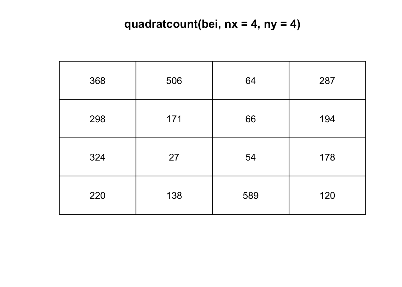

Then predict the intensity based on this function.

prh <- predict(rh)
plot(prh, main = "")
plot(bei, add = TRUE, cols = "white", cex = 0.2, pch = 16)

Contrast this to a simply kernel density estimate without a covariate:

dbei <- density(bei)
plot(dbei, main = "")
plot(bei, add = TRUE, cols = "white", cex = 0.2, pch = 16)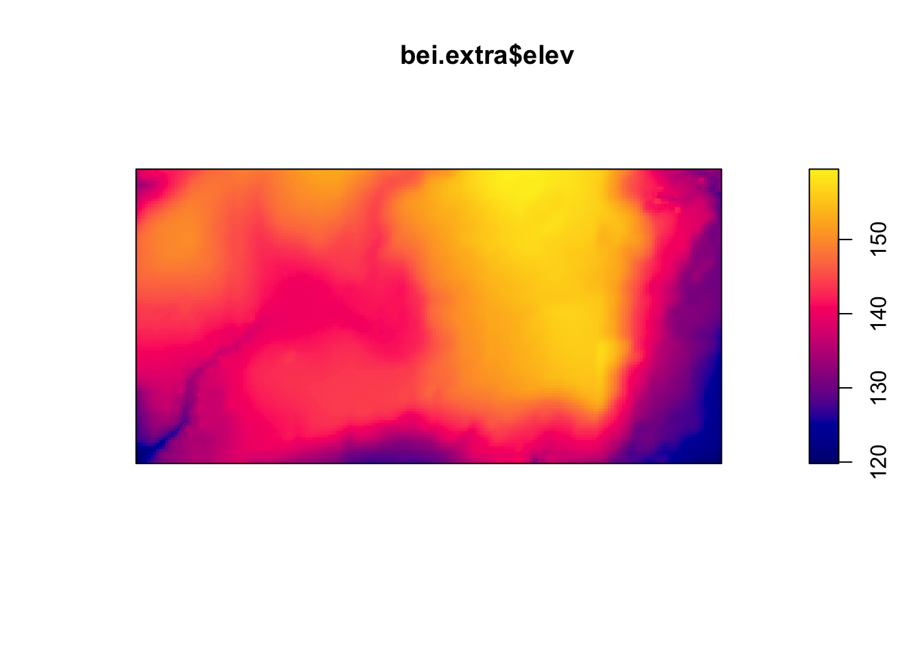

par(mfrow = c(1, 2))
plot(prh, main = "With Covariate")
plot(dbei, main = "Without Covariate")

7.2.3 Parametric Intensity Estimation

Beyond kernel density estimates, we may want to model this intensity with a parametric model. We’ll use a log-link function between the linear model and our intensity.

For a uniform Poisson process, we assume \(log(\lambda(s)) = \beta_0\).

ppm(bei ~ 1)

## Stationary Poisson process
## Intensity: 0.007208
##             Estimate    S.E. CI95.lo CI95.hi Ztest   Zval
## log(lambda)   -4.933 0.01666  -4.965    -4.9   *** -296.1

We may think that the x coordinate linearly impacts the intensity, \(log(\lambda(s)) = \beta_0 + \beta_1 x\).

ppm(bei ~ x)

## Nonstationary Poisson process
## 
## Log intensity:  ~x
## 
## Fitted trend coefficients:
## (Intercept)           x 
##  -4.5577339  -0.0008031 
## 
##               Estimate      S.E.   CI95.lo    CI95.hi Ztest   Zval
## (Intercept) -4.5577339 3.040e-02 -4.617323 -4.4981449   *** -149.9
## x           -0.0008031 5.863e-05 -0.000918 -0.0006882   ***  -13.7

We may think that the x and y coordinates linearly impact the intensity, \(log(\lambda(s)) = \beta_0 + \beta_1 x + \beta_2 y\).

ppm(bei ~ x + y)

## Nonstationary Poisson process
## 
## Log intensity:  ~x + y
## 
## Fitted trend coefficients:
## (Intercept)           x           y 
##  -4.7245290  -0.0008031   0.0006496 
## 
##               Estimate      S.E.    CI95.lo    CI95.hi Ztest     Zval
## (Intercept) -4.7245290 4.306e-02 -4.8089234 -4.6401346   *** -109.722
## x           -0.0008031 5.863e-05 -0.0009180 -0.0006882   ***  -13.698
## y            0.0006496 1.157e-04  0.0004228  0.0008764   ***    5.614

We could use a variety of models based solely on the x and y coordinates of their location:

(mod <- ppm(bei ~ polynom(x, y, 2)))  #quadratic relationship

## Nonstationary Poisson process
## 
## Log intensity:  ~x + y + I(x^2) + I(x * y) + I(y^2)
## 
## Fitted trend coefficients:
## (Intercept)           x           y      I(x^2)    I(x * y) 
##  -4.276e+00  -1.609e-03  -4.895e-03   1.626e-06  -2.836e-06 
##      I(y^2) 
##   1.331e-05 
## 
##               Estimate      S.E.    CI95.lo    CI95.hi Ztest    Zval
## (Intercept) -4.276e+00 7.811e-02 -4.429e+00 -4.123e+00   *** -54.739
## x           -1.609e-03 2.441e-04 -2.088e-03 -1.131e-03   ***  -6.593
## y           -4.895e-03 4.839e-04 -5.844e-03 -3.947e-03   *** -10.116
## I(x^2)       1.626e-06 2.197e-07  1.195e-06  2.057e-06   ***   7.400
## I(x * y)    -2.836e-06 3.511e-07 -3.525e-06 -2.148e-06   ***  -8.078
## I(y^2)       1.331e-05 8.488e-07  1.165e-05  1.498e-05   ***  15.686

(mod1 <- ppm(bei ~ I(x > 50)))  #threshold

## Nonstationary Poisson process
## 
## Log intensity:  ~I(x > 50)
## 
## Fitted trend coefficients:
##   (Intercept) I(x > 50)TRUE 
##       -4.3790       -0.5961 
## 
##               Estimate    S.E. CI95.lo CI95.hi Ztest   Zval
## (Intercept)    -4.3790 0.05472 -4.4863 -4.2718   *** -80.03
## I(x > 50)TRUE  -0.5961 0.05744 -0.7086 -0.4835   *** -10.38

require(splines)
(mod2 <- ppm(bei ~ bs(x) + bs(y)))  #B-spline

## Nonstationary Poisson process
## 
## Log intensity:  ~bs(x) + bs(y)
## 
## Fitted trend coefficients:
## (Intercept)      bs(x)1      bs(x)2      bs(x)3      bs(y)1 
##    -3.49663    -2.04026    -0.23164    -1.36342    -1.79118 
##      bs(y)2      bs(y)3 
##    -0.57816    -0.05631 
## 
##             Estimate    S.E. CI95.lo  CI95.hi Ztest     Zval
## (Intercept) -3.49663 0.07468 -3.6430 -3.35025   *** -46.8211
## bs(x)1      -2.04026 0.17103 -2.3755 -1.70505   *** -11.9295
## bs(x)2      -0.23164 0.12980 -0.4860  0.02277        -1.7845
## bs(x)3      -1.36342 0.10227 -1.5639 -1.16297   *** -13.3311
## bs(y)1      -1.79118 0.18113 -2.1462 -1.43617   ***  -9.8888
## bs(y)2      -0.57816 0.11816 -0.8097 -0.34657   ***  -4.8931
## bs(y)3      -0.05631 0.08836 -0.2295  0.11687        -0.6373

plot(predict(mod))

plot(predict(mod1))

plot(predict(mod2))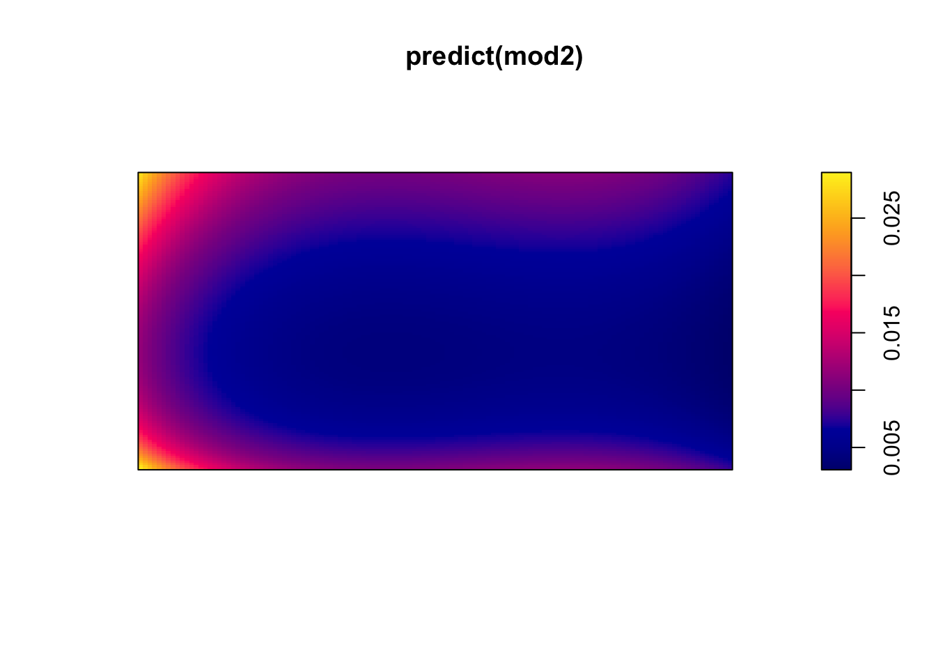

We can compare models using a likelihood ratio test.

hom <- ppm(bei ~ 1)

anova(hom, mod, test = "Chi")

## Analysis of Deviance Table
## 
## Model 1: ~1   Poisson
## Model 2: ~x + y + I(x^2) + I(x * y) + I(y^2)      Poisson
##   Npar Df Deviance Pr(>Chi)    
## 1    1                         
## 2    6  5      604   <2e-16 ***
## ---
## Signif. codes:  0 '***' 0.001 '**' 0.01 '*' 0.05 '.' 0.1 ' ' 1

Also, considering the residuals, we should look to see if there is a pattern in where our model has errors in predicting the intensity.

diagnose.ppm(mod, which = "smooth")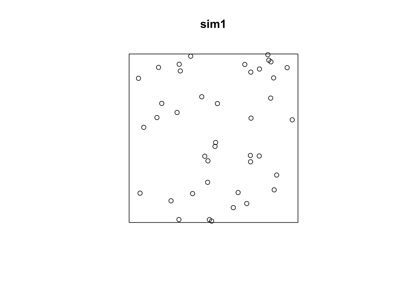

## Model diagnostics (raw residuals)
## Diagnostics available:
##  smoothed residual field
## range of smoothed field =  [-0.004988, 0.006086]

As we saw with the kernel density estimation, the elevation plays a role in the intensity of trees. Let’s add that into our model,

\[\log(\lambda(s)) = \beta_0 + \beta_1 Elevation(s)\]

(mod2 <- ppm(bei ~ elev))

## Nonstationary Poisson process
## 
## Log intensity:  ~elev
## 
## Fitted trend coefficients:
## (Intercept)        elev 
##    -5.63919     0.00489 
## 
##             Estimate     S.E.    CI95.lo  CI95.hi Ztest    Zval
## (Intercept) -5.63919 0.304566 -6.2361283 -5.04225   *** -18.516
## elev         0.00489 0.002102  0.0007696  0.00901     *   2.326

diagnose.ppm(mod2, which = "smooth")

## Model diagnostics (raw residuals)
## Diagnostics available:
##  smoothed residual field
## range of smoothed field =  [-0.004413, 0.007798]

plot(effectfun(mod2))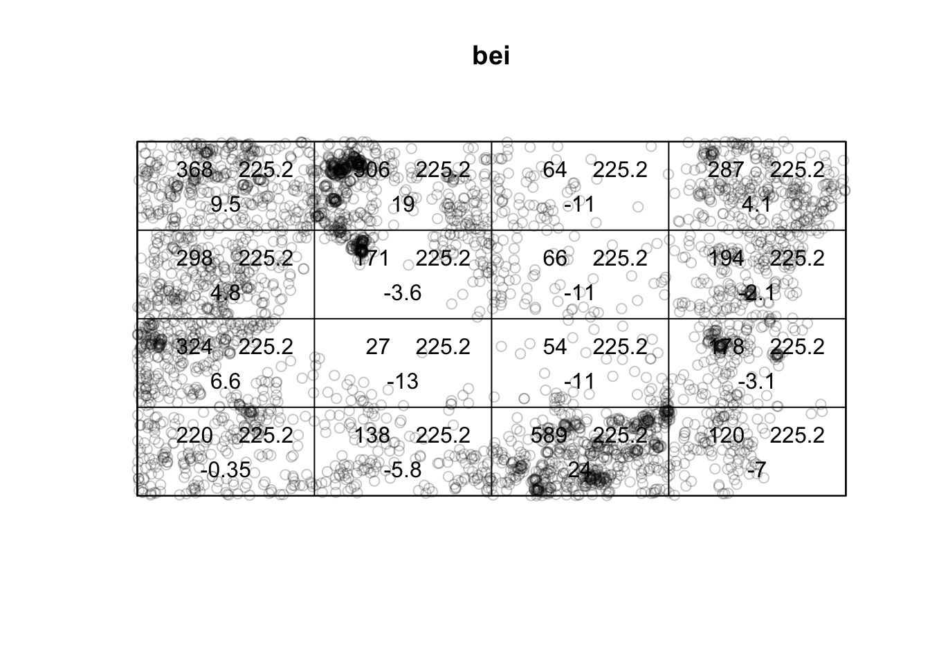

But the relationship may not be linear, so let’s try a quadratic relationship with elevation,

\[\log(\lambda(s)) = \beta_0 + \beta_1 Elevation(s)+ \beta_2 Elevation^2(s)\]

(mod2 <- ppm(bei ~ polynom(elev, 2)))

## Nonstationary Poisson process
## 
## Log intensity:  ~elev + I(elev^2)
## 
## Fitted trend coefficients:
## (Intercept)        elev   I(elev^2) 
##  -1.380e+02   1.847e+00  -6.396e-03 
## 
##               Estimate      S.E.    CI95.lo    CI95.hi Ztest   Zval
## (Intercept) -1.380e+02 6.7047210 -1.511e+02 -1.248e+02   *** -20.58
## elev         1.847e+00 0.0927883  1.665e+00  2.029e+00   ***  19.91
## I(elev^2)   -6.396e-03 0.0003208 -7.025e-03 -5.767e-03   *** -19.94

diagnose.ppm(mod2, which = "smooth")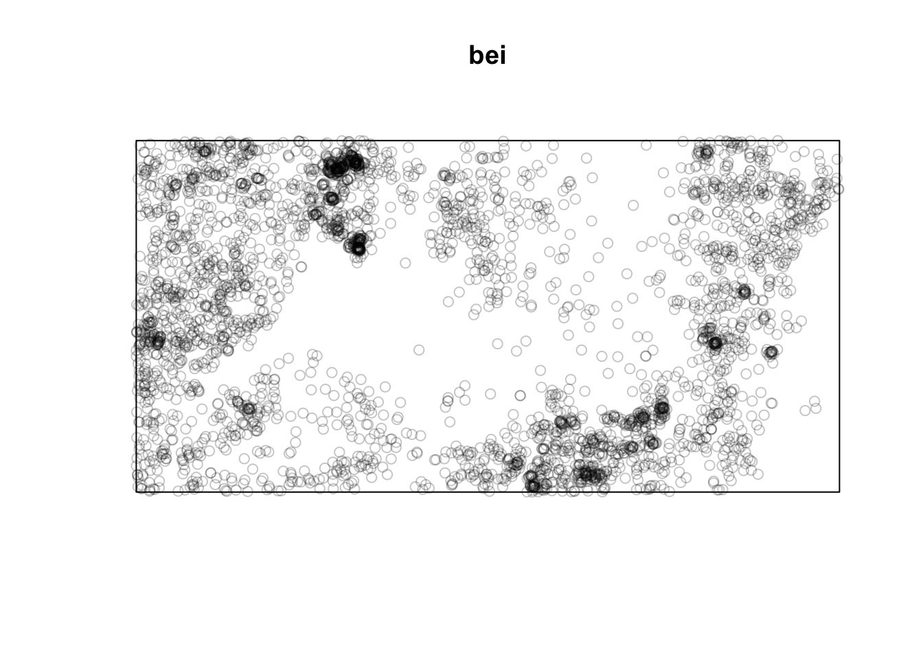

## Model diagnostics (raw residuals)
## Diagnostics available:
##  smoothed residual field
## range of smoothed field =  [-0.005641, 0.006091]

plot(effectfun(mod2))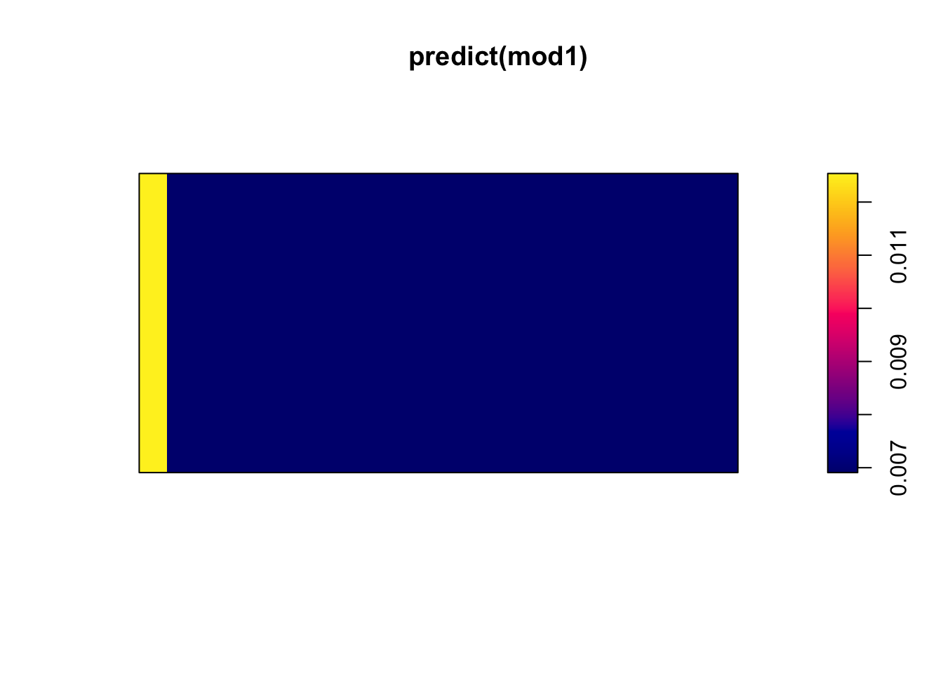

7.2.4 Detecting Interaction Effects

Classical tests about the interaction effects between points are based on derived distances.

Pairwise distances: \(d_{ij} = ||s_i - s_j||\) (pairdist)

pairdist(bei)[1:10, 1:10]  #distance matrix for each pair of points

##         [,1]    [,2]    [,3]    [,4]   [,5]   [,6]   [,7]   [,8]
##  [1,]    0.0 1025.98 1008.74 1012.77 969.05 964.32 973.10 959.12
##  [2,] 1026.0    0.00   19.04   13.26  56.92  61.76  54.03  71.28
##  [3,] 1008.7   19.04    0.00   10.01  40.43  45.85  40.32  59.22
##  [4,] 1012.8   13.26   10.01    0.00  43.73  48.51  40.88  58.55
##  [5,]  969.1   56.92   40.43   43.73   0.00   5.92  11.60  26.11
##  [6,]  964.3   61.76   45.85   48.51   5.92   0.00  11.41  21.20
##  [7,]  973.1   54.03   40.32   40.88  11.60  11.41   0.00  19.35
##  [8,]  959.1   71.28   59.22   58.55  26.11  21.20  19.35   0.00
##  [9,]  961.4   73.63   63.88   61.62  35.33  31.01  26.46  10.51
## [10,]  928.8  158.88  154.57  149.58 128.72 123.70 120.34 102.62
##         [,9]  [,10]
##  [1,] 961.40 928.81
##  [2,]  73.63 158.88
##  [3,]  63.88 154.57
##  [4,]  61.62 149.58
##  [5,]  35.33 128.72
##  [6,]  31.01 123.70
##  [7,]  26.46 120.34
##  [8,]  10.51 102.62
##  [9,]   0.00  93.91
## [10,]  93.91   0.00

Nearest neighbor distances: \(t_i = \min_{j\not= i} d_{ij}\) (nndist)

mean(nndist(bei))  #average first nearest neighbor distance

## [1] 4.33

mean(nndist(bei, k = 2))  #average second nearest neighbor distance

## [1] 6.473

ANN <- apply(nndist(bei, k = 1:100), 2, mean)  #Mean for 1,...,100 nearest neighbors
plot(ANN ~ I(1:100), type = "b", main = NULL, las = 1)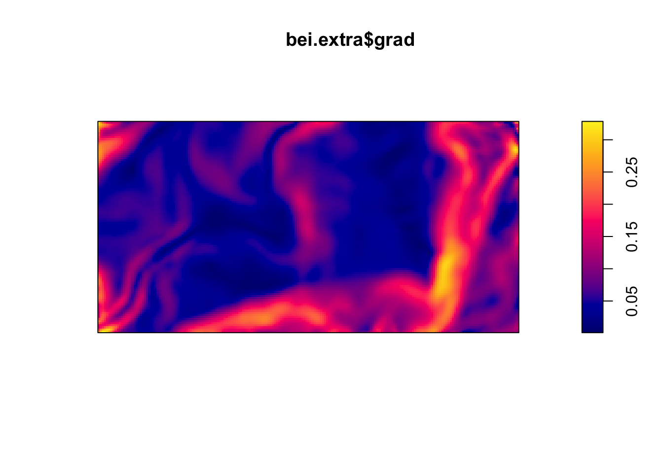

Empty space distances: \(d(u) = \min_{i}||u- s_i||\), the distance from a fixed reference location \(u\) in the the window to the nearest data point (distmap)

plot(distmap(bei))  #map of the distances to the nearest observed point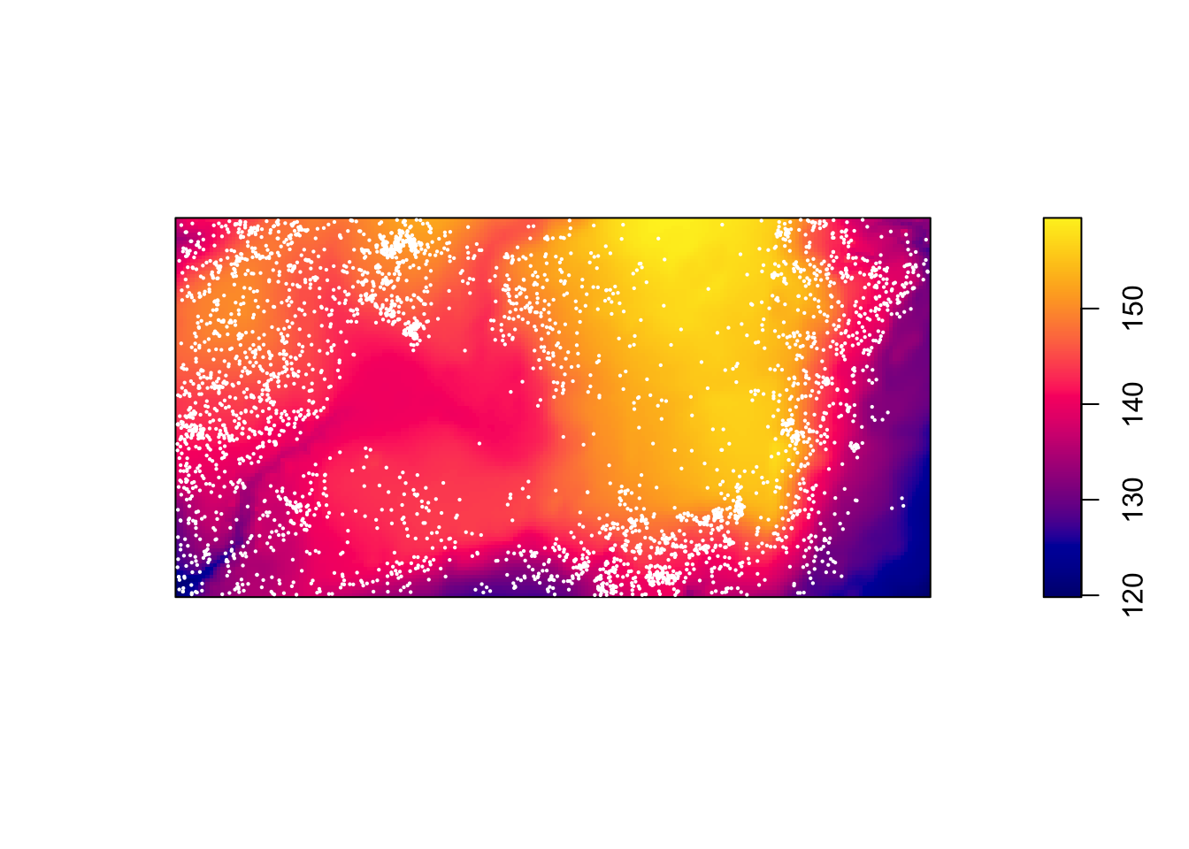

7.2.4.1 F function

Consider the empty-space distance.

Fix the observation window \(A\). The distribution of \(d(u)\), the minimum distance to an observed point, depends on \(A\) and it is hard to derive in closed form.

Consider the CDF,

\[F_u(r) = P(d(u) \leq r)\] \[= P(\text{ at least one point within radius }r\text{ of }u)\] \[= 1 - P(\text{ no points within radius }r\text{ of }u)\]

For a homogeneous Poisson process on \(R^2\),

\[F(r) = 1 - e^{-\lambda \pi r^2}\]

Consider the process defined on \(R^2\) and we only observe it on \(A\). The observed distances are biased relative to the “true” distances, which result in “edge effects”.
If you define a set of locations \(u_1,...,u_m\) for estimating \(F(r)\) under an assumption of statitionary, the estimator

\[\hat{F}(r) = \frac{1}{m} \sum^m_{j=1}I(d(u_j)\leq r)\]

is biased due to the edge effects.

There are a variety of corrections.
- One example is to not consider \(u\)’s within distance \(r\) of the boundary (border correction).
- Another example is to consider it a censored data problem and use a spatial varient of the Kaplan-Meier correction.

Compare the \(\hat{F}(r)\) to the \(F(r)\) under a homogenous Poisson process.

plot(Fest(bei))  #km is kaplan meier correction, bord is the border correction (reduced sample)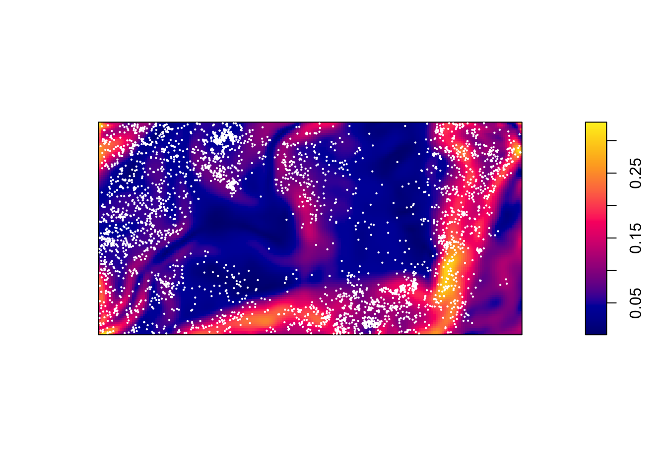

In this plot, we observe fewer short distances than what we’d expect if it were a completely random Poisson point process (\(F_{pois}\)) and thus many more longer distances to observed points. Thus, there are more spots that don’t have many points (larger distances to observed points), meaning points are more clustered than what you’d expect from a uniform distribution across the space.

7.2.4.2 G function

Working instead with the nearest-neighbor distances from points themselves (\(t_i = \min_{j\not= i} d_{ij}\)), we define

\[G(r) = P(t_i \leq r)\] for an arbitrary observed point \(s_i\). We can estimate it using our observed \(t_i\)’s.

\[\hat{G}(r) = \frac{1}{n}\sum^n_{i=1}I(t_i \leq r)\]

As before, we may or may not make an edge correction.

For a homogeneous Poisson process on \(R^2\),

\[G(r) = 1 - e^{-\lambda \pi r^2}\]

Compare the \(\hat{G}(r)\) to the \(G(r)\) under a homogenous Poisson process.

plot(Gest(bei))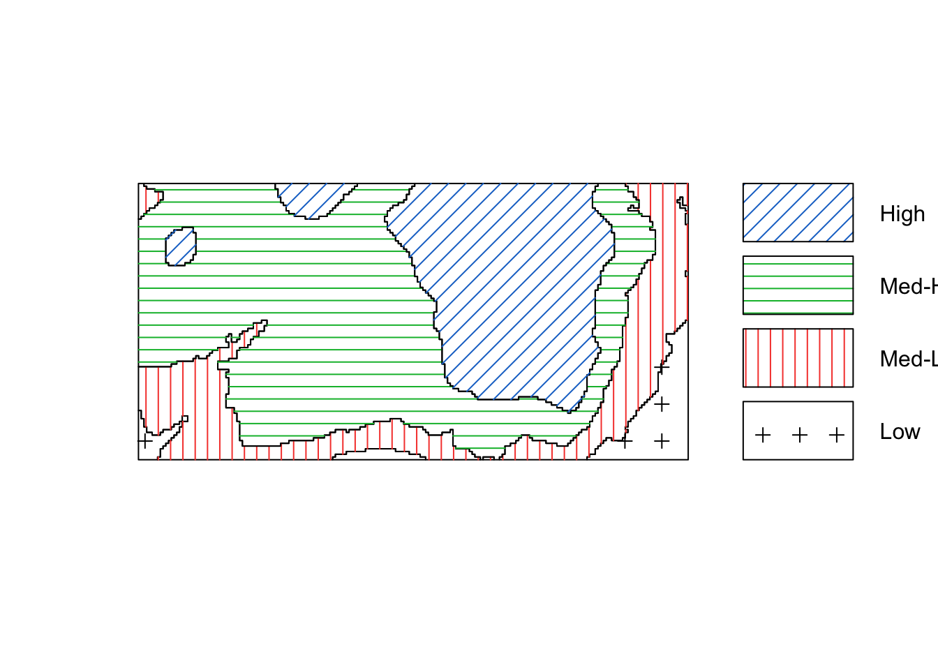

Here we observe that we see more short nearest neighbor distances than what we’d expect if it were a completely random Poisson point process. Thus, the points are more clustered than what you’d expect from a uniform distribution across the space.

7.2.4.3 K function

Another approach is to consider Ripley’s K function, which summarizes the distance between points. It consists of dividing the mean of the total number of points at different distance lags from each point by the area event density. In other words, it is concerned with the number of events falling within a circle of radius \(r\) of an event.

\[K(r) = \frac{1}{\lambda}E(\text{ points within distance r of an arbitrary point})\]

Under CSR (uniform intensity), we’d expect \(K(r) = \pi r^2\) because that is the area of the circle. Points that cluster more than you’d expect corresponds to \(K(r) > \pi r^2\) and spatial repulsion corresponds to \(K(r) < \pi r^2\).

Below, we have an estimate of the K function (black solid) along with the predicted K function if \(H_0\) were true (red dashed). For this set of trees, the points are more clustered than you’d expect for an homogenous Poisson process.

plot(Kest(bei))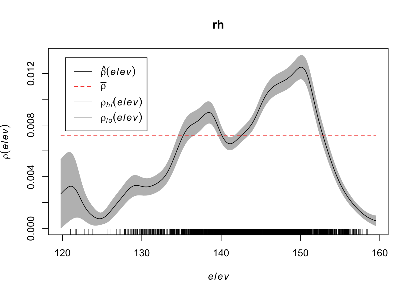

7.2.4.4 L function

It is hard to see differences between the estimated \(K\) function and the expected function. An alternative is to transform the values such that the expected values is a horizontal line The transofmration is calculated as follows:

\[L(r) = \sqrt{K(r)/\pi} - d\]

plot(Kest(bei), sqrt(./pi) - r ~ r)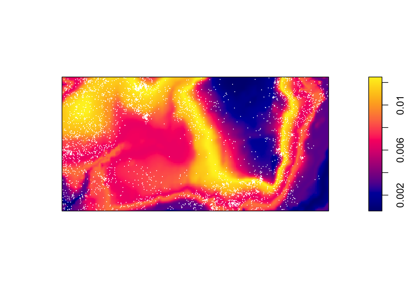

7.2.4.5 Pair Correlation Function

The second-order intensity function is

\[\lambda_2(s_1,s_2) = \lim_{|ds_1|,|ds_2| \rightarrow 0} \frac{E[N(ds_1)N(ds_2)]}{|ds_1||ds_2|}\]

where \(s_1 \not= s_2\). If \(\lambda(s)\) is constant and

\[\lambda_2(s_1,s_2) = \lambda_2(s_1 - s_2) =\lambda_2(s_2 - s_1)\] then we call \(N\) second-order stationary.

We can define \(g\) as the pair correlation function (PCF),

\[g(s_1,s_2) = \frac{\lambda_2(s_1,s_2)}{\lambda(s_1)\lambda(s_2)}\]

In R, if we assume stationarity and isotropy (direction of distance is not important), we can estimate \(g(r)\) where \(r = ||s_1-s_2||\). If a process has an isotropic pair correlation function, then our K function can be defined as

\[K(r) = 2\pi \int^r_0 ug(u)du, r>0\]

plot(pcf(bei))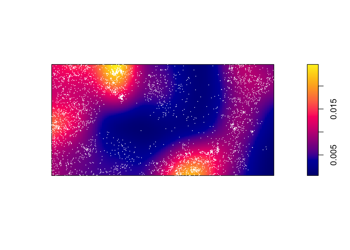

If \(g(r) = 1\), then we have a CSR process. If \(g(r)> 1\), it implies a cluster process and if \(g(r)<1\), it implies an inhibition process. In particular, if \(g(r) = 0\) for \(r_i<r\), it implies a hard core processes (no point pairs within this distance).

7.2.4.6 Envelopes

We want to test \(H_0\): CSR (constant intensity) to get a sense of whether points are closer or further away from each other than we’d expect with a Poisson process.

For any of these 3 (4) functions, we can compare the estimated function to the theoretical but that doesn’t tell us how far our estimate might be from the truth under random variability. So we can simulate under our null hypothesis (CSR) say \(B\) times and for each time, we estimate the function. Then we create a single global test:

\[D_i = \max_r |\hat{H}_i(r) - H(r)|,\quad i=1,...,B\]

where \(H(r)\) is the theoretical value under CSR. Then we define \(D_{crit}\) to be the \(k\)th largest among the \(D_i\). The “global” envelopes are then

\[L(r) = H(r) - D_{crit}\] \[U(r) = H(r) + D_{crit}\]

Then the test that rejects \(\hat{H}_1\) (estimate from our observations) ever wanders outside \((L(r), U(r))\) has size \(\alpha = 1 - k/B\).

plot(envelope(bei, Fest, global = TRUE))

## Generating 99 simulations of CSR  ...
## 1, 2, 3, 4, 5, 6, 7, 8, 9, 10, 11, 12, 13, 14, 15, 16, 17, 18, 19, 20, 21, 22, 23, 24, 25, 26, 27, 28, 29, 30, 31, 32, 33, 34, 35,
## 36, 37, 38, 39, 40, 41, 42, 43, 44, 45, 46, 47, 48, 49, 50, 51, 52, 53, 54, 55, 56, 57, 58, 59, 60, 61, 62, 63, 64, 65, 66, 67, 68, 69, 70,
## 71, 72, 73, 74, 75, 76, 77, 78, 79, 80, 81, 82, 83, 84, 85, 86, 87, 88, 89, 90, 91, 92, 93, 94, 95, 96, 97, 98,  99.
## 
## Done.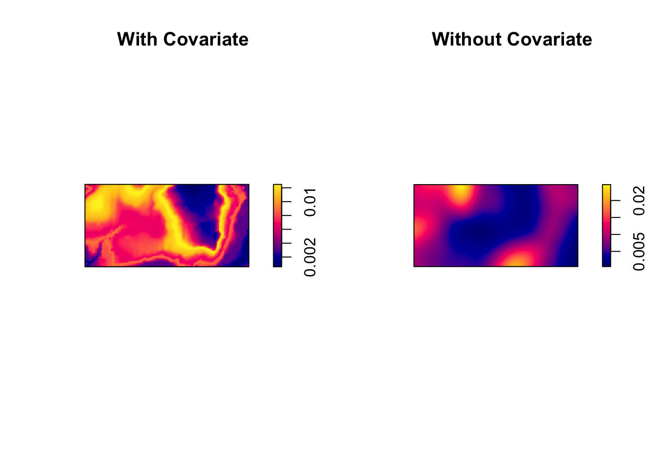

plot(envelope(bei, Gest, global = TRUE))

## Generating 99 simulations of CSR  ...
## 1, 2, 3, 4, 5, 6, 7, 8, 9, 10, 11, 12, 13, 14, 15, 16, 17, 18, 19, 20, 21, 22, 23, 24, 25, 26, 27, 28, 29, 30, 31, 32, 33, 34, 35,
## 36, 37, 38, 39, 40, 41, 42, 43, 44, 45, 46, 47, 48, 49, 50, 51, 52, 53, 54, 55, 56, 57, 58, 59, 60, 61, 62, 63, 64, 65, 66, 67, 68, 69, 70,
## 71, 72, 73, 74, 75, 76, 77, 78, 79, 80, 81, 82, 83, 84, 85, 86, 87, 88, 89, 90, 91, 92, 93, 94, 95, 96, 97, 98,  99.
## 
## Done.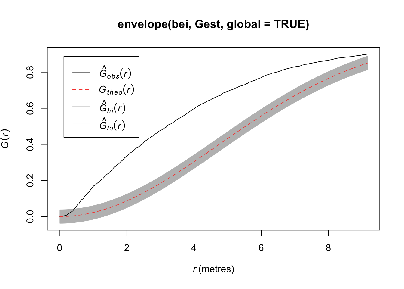

plot(envelope(bei, Kest, global = TRUE))

## Generating 99 simulations of CSR  ...
## 1, 2, 3, 4, 5, 6, 7, 8, 9, 10, 11, 12, 13, 14, 15, 16, 17, 18, 19, 20, 21, 22, 23, 24, 25, 26, 27, 28, 29, 30, 31, 32, 33, 34, 35,
## 36, 37, 38, 39, 40, 41, 42, 43, 44, 45, 46, 47, 48, 49, 50, 51, 52, 53, 54, 55, 56, 57, 58, 59, 60, 61, 62, 63, 64, 65, 66, 67, 68, 69, 70,
## 71, 72, 73, 74, 75, 76, 77, 78, 79, 80, 81, 82, 83, 84, 85, 86, 87, 88, 89, 90, 91, 92, 93, 94, 95, 96, 97, 98,  99.
## 
## Done.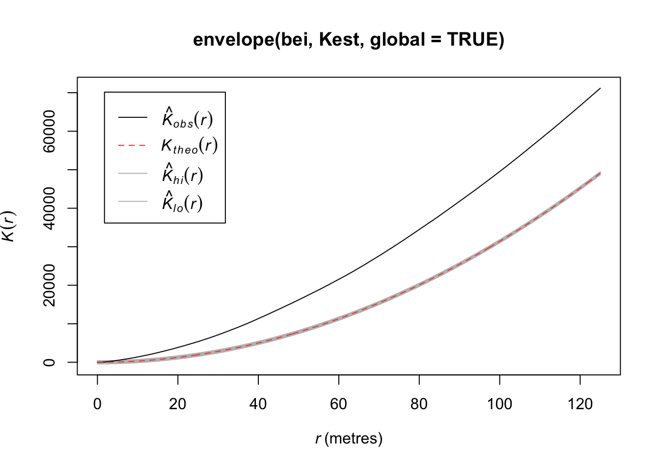

plot(envelope(bei, Lest, global = TRUE))

## Generating 99 simulations of CSR  ...
## 1, 2, 3, 4, 5, 6, 7, 8, 9, 10, 11, 12, 13, 14, 15, 16, 17, 18, 19, 20, 21, 22, 23, 24, 25, 26, 27, 28, 29, 30, 31, 32, 33, 34, 35,
## 36, 37, 38, 39, 40, 41, 42, 43, 44, 45, 46, 47, 48, 49, 50, 51, 52, 53, 54, 55, 56, 57, 58, 59, 60, 61, 62, 63, 64, 65, 66, 67, 68, 69, 70,
## 71, 72, 73, 74, 75, 76, 77, 78, 79, 80, 81, 82, 83, 84, 85, 86, 87, 88, 89, 90, 91, 92, 93, 94, 95, 96, 97, 98,  99.
## 
## Done.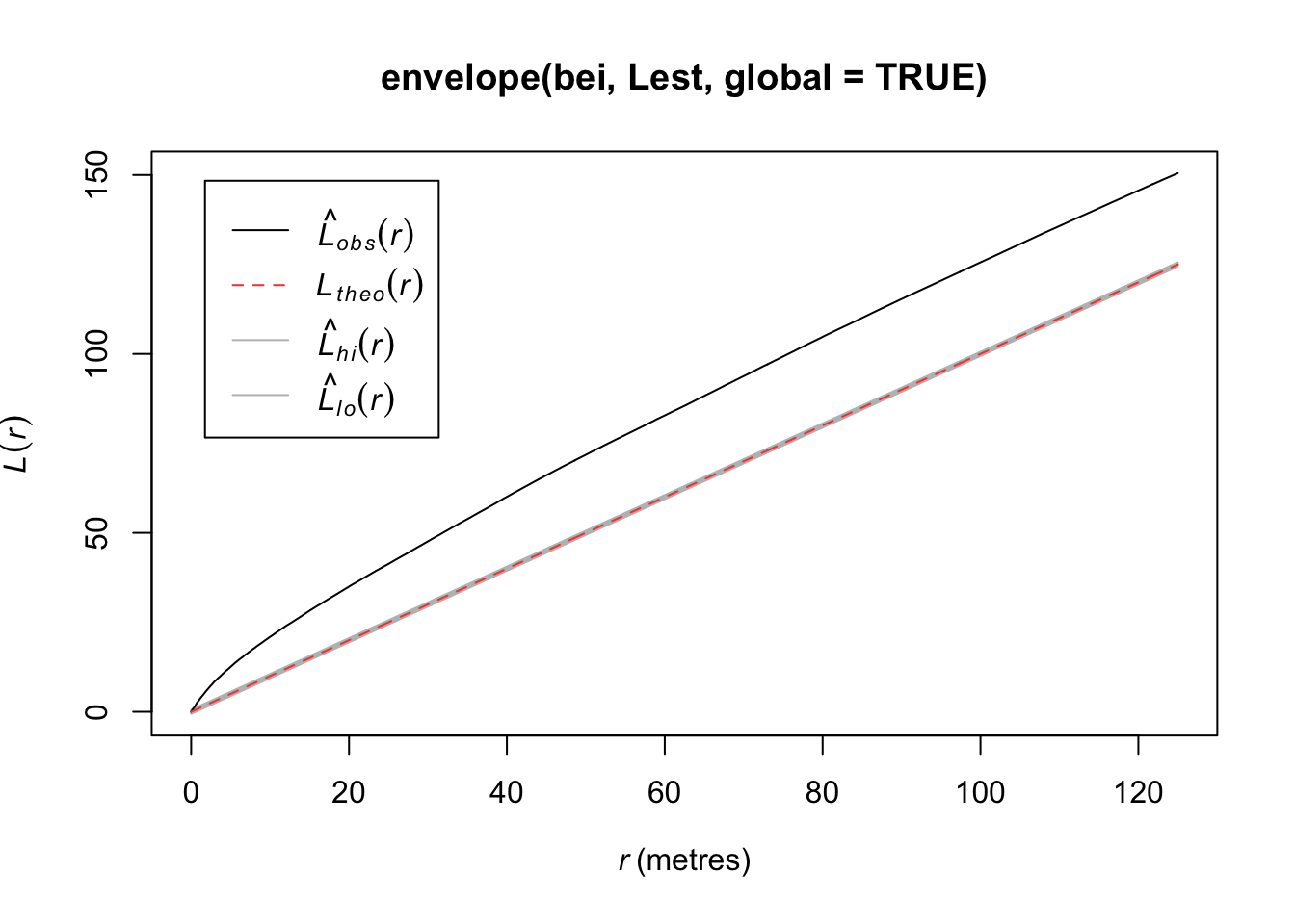

plot(envelope(bei, pcf, global = TRUE))

## Generating 99 simulations of CSR  ...
## 1, 2,  [etd 4:48] 3,
##  [etd 4:57] 4,  [etd 4:56] 5,  [etd 5:07] 6,
##  [etd 4:59] 7,  [etd 4:54] 8,  [etd 4:47] 9,
##  [etd 4:45] 10,  [etd 4:43] 11,  [etd 4:39] 12,
##  [etd 4:37] 13,  [etd 4:32] 14,  [etd 4:27] 15,
##  [etd 4:25] 16,  [etd 4:22] 17,  [etd 4:18] 18,
##  [etd 4:16] 19,  [etd 4:11] 20,  [etd 4:10] 21,
##  [etd 4:05] 22,  [etd 4:00] 23,  [etd 3:56] 24,
##  [etd 3:50] 25,  [etd 3:48] 26,  [etd 3:43] 27,
##  [etd 3:39] 28,  [etd 3:34] 29,  [etd 3:30] 30,
##  [etd 3:27] 31,  [etd 3:23] 32,  [etd 3:19] 33,
##  [etd 3:15] 34,  [etd 3:11] 35,  [etd 3:08] 36,
##  [etd 3:05] 37,  [etd 3:02] 38,  [etd 2:59] 39,
##  [etd 2:55] 40,  [etd 2:53] 41,  [etd 2:50] 42,
##  [etd 2:48] 43,  [etd 2:45] 44,  [etd 2:42] 45,
##  [etd 2:39] 46,  [etd 2:36] 47,  [etd 2:33] 48,
##  [etd 2:31] 49,  [etd 2:27] 50,  [etd 2:24] 51,
##  [etd 2:21] 52,  [etd 2:18] 53,  [etd 2:16] 54,
##  [etd 2:13] 55,  [etd 2:10] 56,  [etd 2:07] 57,
##  [etd 2:04] 58,  [etd 2:01] 59,  [etd 1:58] 60,
##  [etd 1:55] 61,  [etd 1:52] 62,  [etd 1:49] 63,
##  [etd 1:46] 64,  [etd 1:43] 65,  [etd 1:40] 66,
##  [etd 1:37] 67,  [etd 1:34] 68,  [etd 1:31] 69,
##  [etd 1:28] 70,  [etd 1:26] 71,  [etd 1:23] 72,
##  [etd 1:20] 73,  [etd 1:17] 74,  [etd 1:14] 75,
##  [etd 1:11] 76,  [etd 1:08] 77,  [etd 1:05] 78,
##  [etd 1:02] 79,  [etd 59 sec] 80,  [etd 56 sec] 81,
##  [etd 53 sec] 82,  [etd 51 sec] 83,  [etd 48 sec] 84,
##  [etd 45 sec] 85,  [etd 42 sec] 86,  [etd 39 sec] 87,
##  [etd 36 sec] 88,  [etd 33 sec] 89,  [etd 30 sec] 90,
##  [etd 27 sec] 91,  [etd 24 sec] 92,  [etd 21 sec] 93,
##  [etd 18 sec] 94,  [etd 15 sec] 95,  [etd 12 sec] 96,
##  [etd 9 sec] 97,  [etd 6 sec] 98,  [etd 3 sec]  99.
## 
## Done.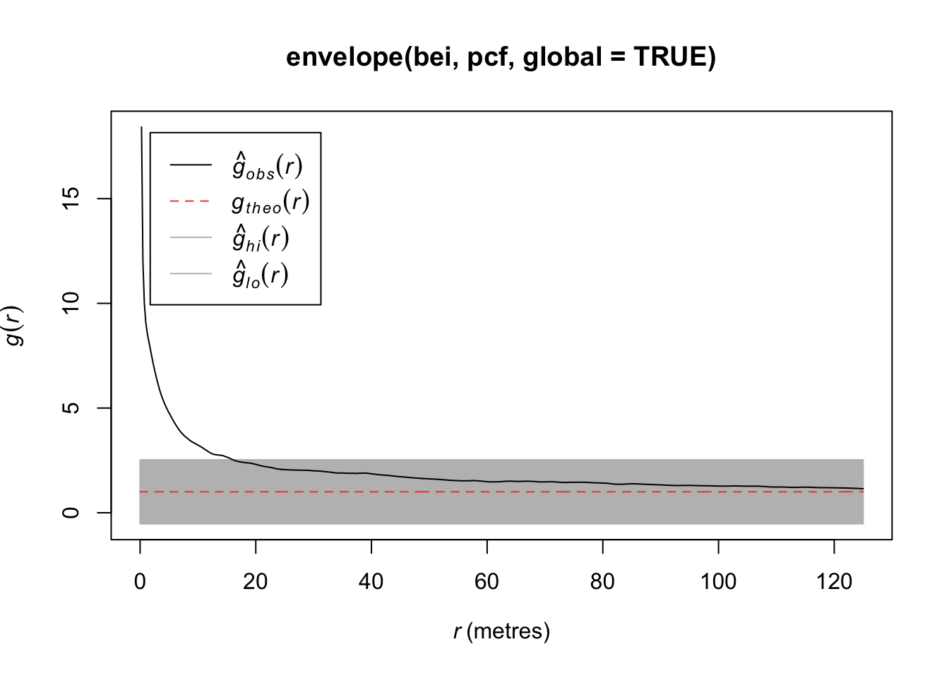

7.2.5 Cluster Poisson Processes

A Poisson cluster process is defined by

Parent events form Poisson process with intensity \(\lambda\).
Each parent produces a random number \(M\) of children, iid for each parent according to a discrete distribution \(p_m\).
The positions of the children relative to parents are iid according to a biviarate pdf.

By convention, the point pattern consists of only the children, not the parents.

7.2.5.1 Matern Process

Homogeneous Poisson parent process with intensity \(\lambda\).
Poisson distributed number of children, mean = \(\mu\)
Children uniformly distributed on disc of radius, \(r\), centered at parent location

Let’s simulate some data from this process.

win <- owin(c(0, 100), c(0, 100))
clust1 <- rMatClust(50/10000, r = 4, mu = 5, win = win)
plot(clust1)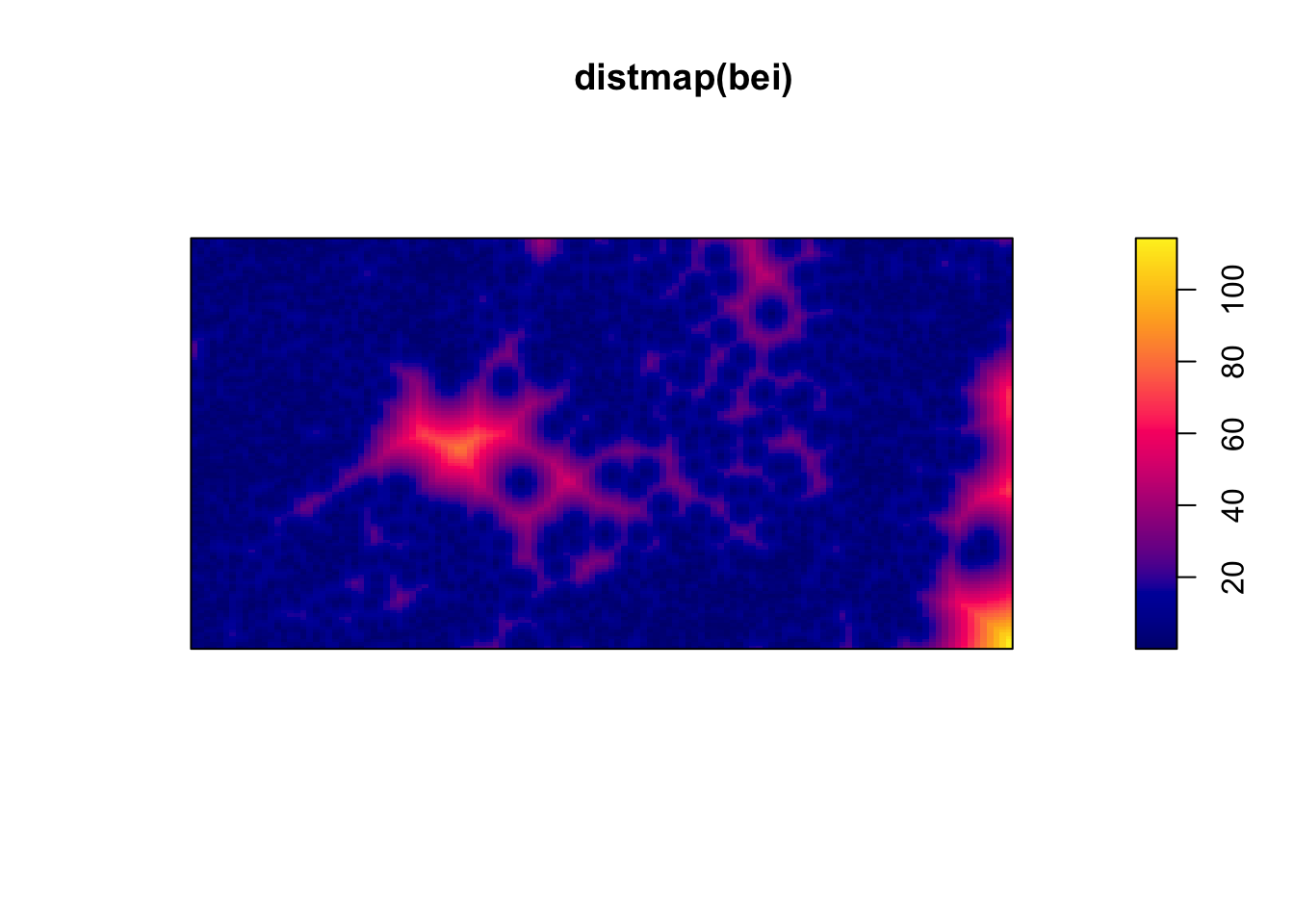

quadrat.test(clust1)

## 
##  Chi-squared test of CSR using quadrat counts
## 
## data:  clust1
## X2 = 207, df = 24, p-value <2e-16
## alternative hypothesis: two.sided
## 
## Quadrats: 5 by 5 grid of tiles

plot(envelope(clust1, Fest, global = TRUE))

## Generating 99 simulations of CSR  ...
## 1, 2, 3, 4, 5, 6, 7, 8, 9, 10, 11, 12, 13, 14, 15, 16, 17, 18, 19, 20, 21, 22, 23, 24, 25, 26, 27, 28, 29, 30, 31, 32, 33, 34, 35,
## 36, 37, 38, 39, 40, 41, 42, 43, 44, 45, 46, 47, 48, 49, 50, 51, 52, 53, 54, 55, 56, 57, 58, 59, 60, 61, 62, 63, 64, 65, 66, 67, 68, 69, 70,
## 71, 72, 73, 74, 75, 76, 77, 78, 79, 80, 81, 82, 83, 84, 85, 86, 87, 88, 89, 90, 91, 92, 93, 94, 95, 96, 97, 98,  99.
## 
## Done.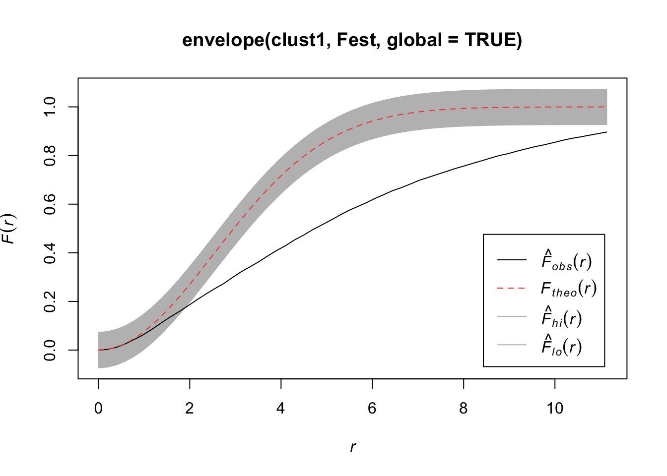

plot(envelope(clust1, Gest, global = TRUE))

## Generating 99 simulations of CSR  ...
## 1, 2, 3, 4, 5, 6, 7, 8, 9, 10, 11, 12, 13, 14, 15, 16, 17, 18, 19, 20, 21, 22, 23, 24, 25, 26, 27, 28, 29, 30, 31, 32, 33, 34, 35,
## 36, 37, 38, 39, 40, 41, 42, 43, 44, 45, 46, 47, 48, 49, 50, 51, 52, 53, 54, 55, 56, 57, 58, 59, 60, 61, 62, 63, 64, 65, 66, 67, 68, 69, 70,
## 71, 72, 73, 74, 75, 76, 77, 78, 79, 80, 81, 82, 83, 84, 85, 86, 87, 88, 89, 90, 91, 92, 93, 94, 95, 96, 97, 98,  99.
## 
## Done.

plot(envelope(clust1, Kest, global = TRUE))

## Generating 99 simulations of CSR  ...
## 1, 2, 3, 4, 5, 6, 7, 8, 9, 10, 11, 12, 13, 14, 15, 16, 17, 18, 19, 20, 21, 22, 23, 24, 25, 26, 27, 28, 29, 30, 31, 32, 33, 34, 35,
## 36, 37, 38, 39, 40, 41, 42, 43, 44, 45, 46, 47, 48, 49, 50, 51, 52, 53, 54, 55, 56, 57, 58, 59, 60, 61, 62, 63, 64, 65, 66, 67, 68, 69, 70,
## 71, 72, 73, 74, 75, 76, 77, 78, 79, 80, 81, 82, 83, 84, 85, 86, 87, 88, 89, 90, 91, 92, 93, 94, 95, 96, 97, 98,  99.
## 
## Done.

plot(envelope(clust1, Lest, global = TRUE))

## Generating 99 simulations of CSR  ...
## 1, 2, 3, 4, 5, 6, 7, 8, 9, 10, 11, 12, 13, 14, 15, 16, 17, 18, 19, 20, 21, 22, 23, 24, 25, 26, 27, 28, 29, 30, 31, 32, 33, 34, 35,
## 36, 37, 38, 39, 40, 41, 42, 43, 44, 45, 46, 47, 48, 49, 50, 51, 52, 53, 54, 55, 56, 57, 58, 59, 60, 61, 62, 63, 64, 65, 66, 67, 68, 69, 70,
## 71, 72, 73, 74, 75, 76, 77, 78, 79, 80, 81, 82, 83, 84, 85, 86, 87, 88, 89, 90, 91, 92, 93, 94, 95, 96, 97, 98,  99.
## 
## Done.

If we increase the radius of space for the children, we won’t notice that it is clustered.

clust2 <- rMatClust(50/10000, r = 40, mu = 5, win = win)
plot(clust2)

quadrat.test(clust2)

## 
##  Chi-squared test of CSR using quadrat counts
## 
## data:  clust2
## X2 = 36, df = 24, p-value = 0.1
## alternative hypothesis: two.sided
## 
## Quadrats: 5 by 5 grid of tiles

plot(envelope(clust2, Fest, global = TRUE))

## Generating 99 simulations of CSR  ...
## 1, 2, 3, 4, 5, 6, 7, 8, 9, 10, 11, 12, 13, 14, 15, 16, 17, 18, 19, 20, 21, 22, 23, 24, 25, 26, 27, 28, 29, 30, 31, 32, 33, 34, 35,
## 36, 37, 38, 39, 40, 41, 42, 43, 44, 45, 46, 47, 48, 49, 50, 51, 52, 53, 54, 55, 56, 57, 58, 59, 60, 61, 62, 63, 64, 65, 66, 67, 68, 69, 70,
## 71, 72, 73, 74, 75, 76, 77, 78, 79, 80, 81, 82, 83, 84, 85, 86, 87, 88, 89, 90, 91, 92, 93, 94, 95, 96, 97, 98,  99.
## 
## Done.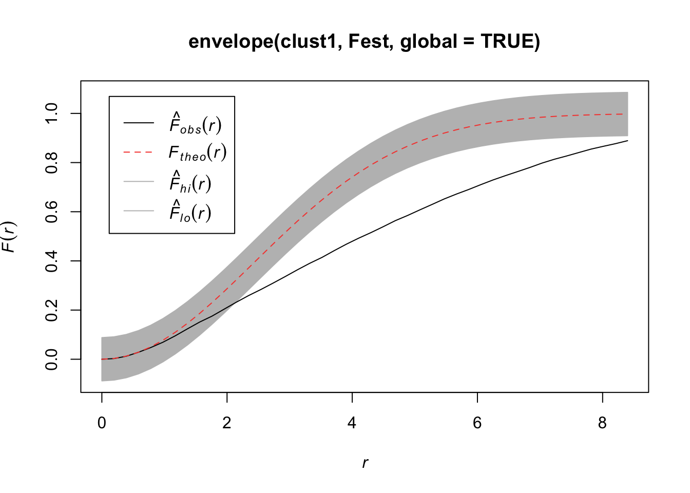

plot(envelope(clust2, Gest, global = TRUE))

## Generating 99 simulations of CSR  ...
## 1, 2, 3, 4, 5, 6, 7, 8, 9, 10, 11, 12, 13, 14, 15, 16, 17, 18, 19, 20, 21, 22, 23, 24, 25, 26, 27, 28, 29, 30, 31, 32, 33, 34, 35,
## 36, 37, 38, 39, 40, 41, 42, 43, 44, 45, 46, 47, 48, 49, 50, 51, 52, 53, 54, 55, 56, 57, 58, 59, 60, 61, 62, 63, 64, 65, 66, 67, 68, 69, 70,
## 71, 72, 73, 74, 75, 76, 77, 78, 79, 80, 81, 82, 83, 84, 85, 86, 87, 88, 89, 90, 91, 92, 93, 94, 95, 96, 97, 98,  99.
## 
## Done.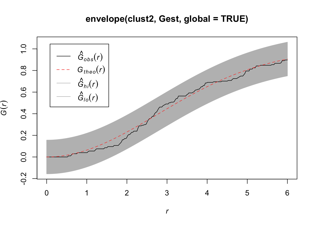

plot(envelope(clust2, Kest, global = TRUE))

## Generating 99 simulations of CSR  ...
## 1, 2, 3, 4, 5, 6, 7, 8, 9, 10, 11, 12, 13, 14, 15, 16, 17, 18, 19, 20, 21, 22, 23, 24, 25, 26, 27, 28, 29, 30, 31, 32, 33, 34, 35,
## 36, 37, 38, 39, 40, 41, 42, 43, 44, 45, 46, 47, 48, 49, 50, 51, 52, 53, 54, 55, 56, 57, 58, 59, 60, 61, 62, 63, 64, 65, 66, 67, 68, 69, 70,
## 71, 72, 73, 74, 75, 76, 77, 78, 79, 80, 81, 82, 83, 84, 85, 86, 87, 88, 89, 90, 91, 92, 93, 94, 95, 96, 97, 98,  99.
## 
## Done.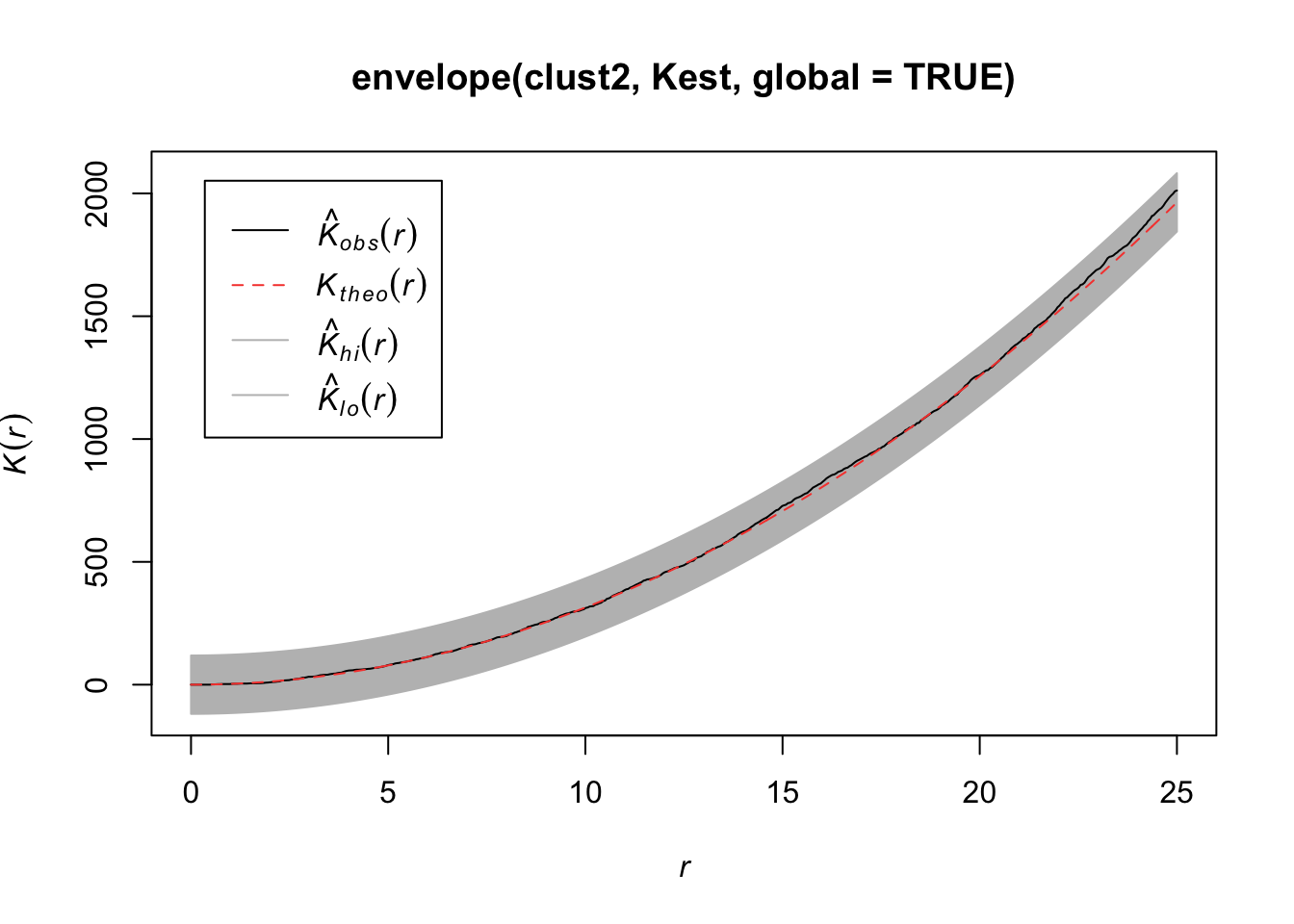

plot(envelope(clust2, Lest, global = TRUE))

## Generating 99 simulations of CSR  ...
## 1, 2, 3, 4, 5, 6, 7, 8, 9, 10, 11, 12, 13, 14, 15, 16, 17, 18, 19, 20, 21, 22, 23, 24, 25, 26, 27, 28, 29, 30, 31, 32, 33, 34, 35,
## 36, 37, 38, 39, 40, 41, 42, 43, 44, 45, 46, 47, 48, 49, 50, 51, 52, 53, 54, 55, 56, 57, 58, 59, 60, 61, 62, 63, 64, 65, 66, 67, 68, 69, 70,
## 71, 72, 73, 74, 75, 76, 77, 78, 79, 80, 81, 82, 83, 84, 85, 86, 87, 88, 89, 90, 91, 92, 93, 94, 95, 96, 97, 98,  99.
## 
## Done.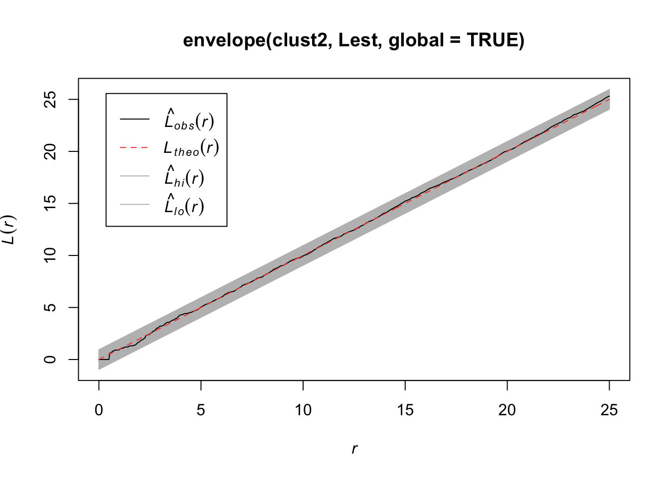

7.2.5.2 Thomas Process

Homogeneous Poisson parent process
Poisson distributed number of children
Locations of children according to isotropic bivariate normal distribution with variance \(\sigma^2\)

clust3 <- rThomas(50/10000, scale = 2, mu = 5, win = win)
plot(clust3)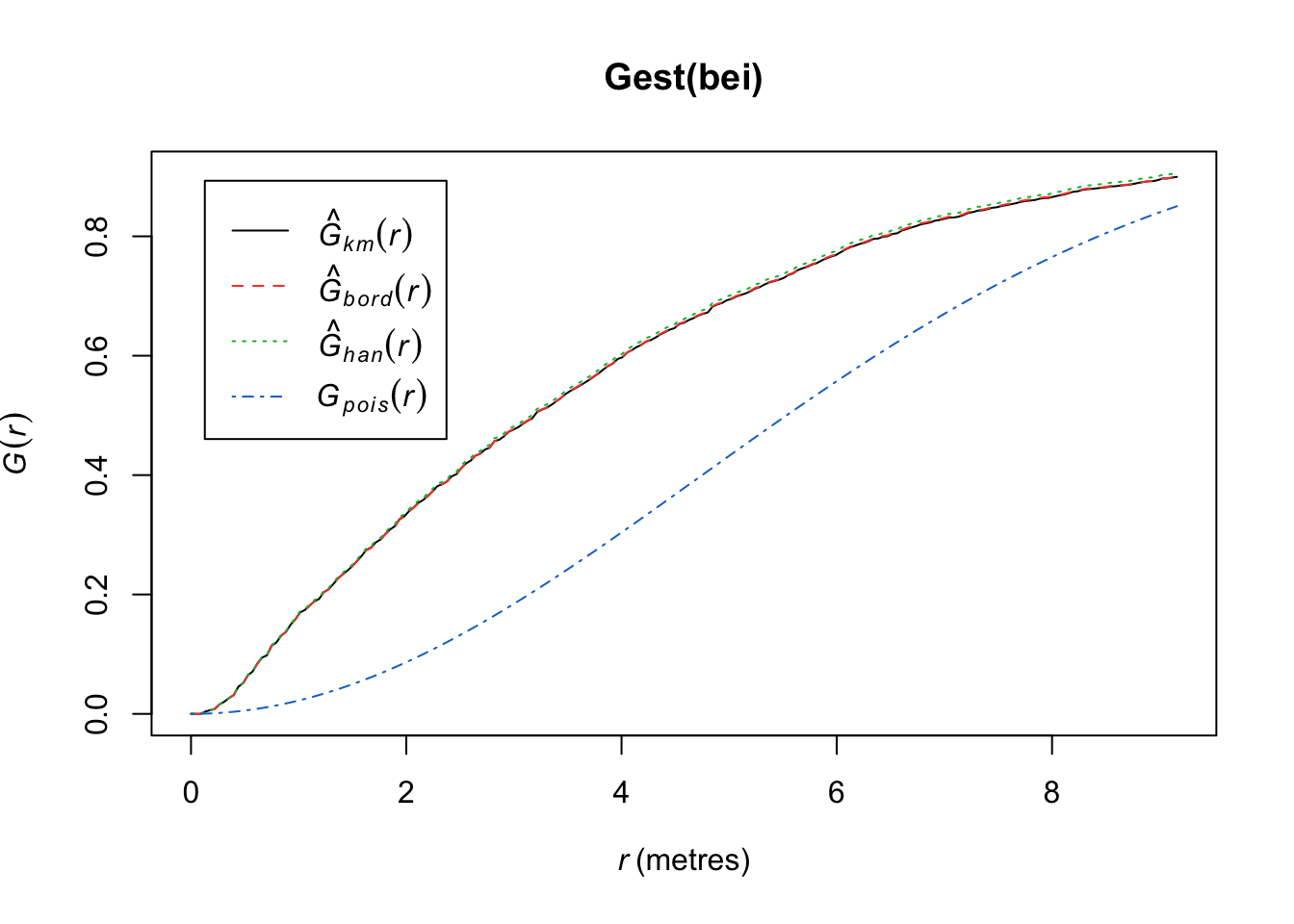

quadrat.test(clust3)

## 
##  Chi-squared test of CSR using quadrat counts
## 
## data:  clust3
## X2 = 112, df = 24, p-value = 4e-13
## alternative hypothesis: two.sided
## 
## Quadrats: 5 by 5 grid of tiles

plot(envelope(clust3, Fest, global = TRUE))

## Generating 99 simulations of CSR  ...
## 1, 2, 3, 4, 5, 6, 7, 8, 9, 10, 11, 12, 13, 14, 15, 16, 17, 18, 19, 20, 21, 22, 23, 24, 25, 26, 27, 28, 29, 30, 31, 32, 33, 34, 35,
## 36, 37, 38, 39, 40, 41, 42, 43, 44, 45, 46, 47, 48, 49, 50, 51, 52, 53, 54, 55, 56, 57, 58, 59, 60, 61, 62, 63, 64, 65, 66, 67, 68, 69, 70,
## 71, 72, 73, 74, 75, 76, 77, 78, 79, 80, 81, 82, 83, 84, 85, 86, 87, 88, 89, 90, 91, 92, 93, 94, 95, 96, 97, 98,  99.
## 
## Done.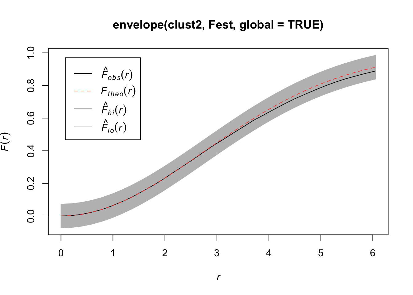

plot(envelope(clust3, Gest, global = TRUE))

## Generating 99 simulations of CSR  ...
## 1, 2, 3, 4, 5, 6, 7, 8, 9, 10, 11, 12, 13, 14, 15, 16, 17, 18, 19, 20, 21, 22, 23, 24, 25, 26, 27, 28, 29, 30, 31, 32, 33, 34, 35,
## 36, 37, 38, 39, 40, 41, 42, 43, 44, 45, 46, 47, 48, 49, 50, 51, 52, 53, 54, 55, 56, 57, 58, 59, 60, 61, 62, 63, 64, 65, 66, 67, 68, 69, 70,
## 71, 72, 73, 74, 75, 76, 77, 78, 79, 80, 81, 82, 83, 84, 85, 86, 87, 88, 89, 90, 91, 92, 93, 94, 95, 96, 97, 98,  99.
## 
## Done.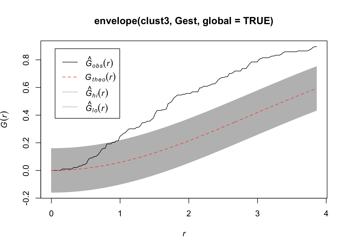

plot(envelope(clust3, Kest, global = TRUE))

## Generating 99 simulations of CSR  ...
## 1, 2, 3, 4, 5, 6, 7, 8, 9, 10, 11, 12, 13, 14, 15, 16, 17, 18, 19, 20, 21, 22, 23, 24, 25, 26, 27, 28, 29, 30, 31, 32, 33, 34, 35,
## 36, 37, 38, 39, 40, 41, 42, 43, 44, 45, 46, 47, 48, 49, 50, 51, 52, 53, 54, 55, 56, 57, 58, 59, 60, 61, 62, 63, 64, 65, 66, 67, 68, 69, 70,
## 71, 72, 73, 74, 75, 76, 77, 78, 79, 80, 81, 82, 83, 84, 85, 86, 87, 88, 89, 90, 91, 92, 93, 94, 95, 96, 97, 98,  99.
## 
## Done.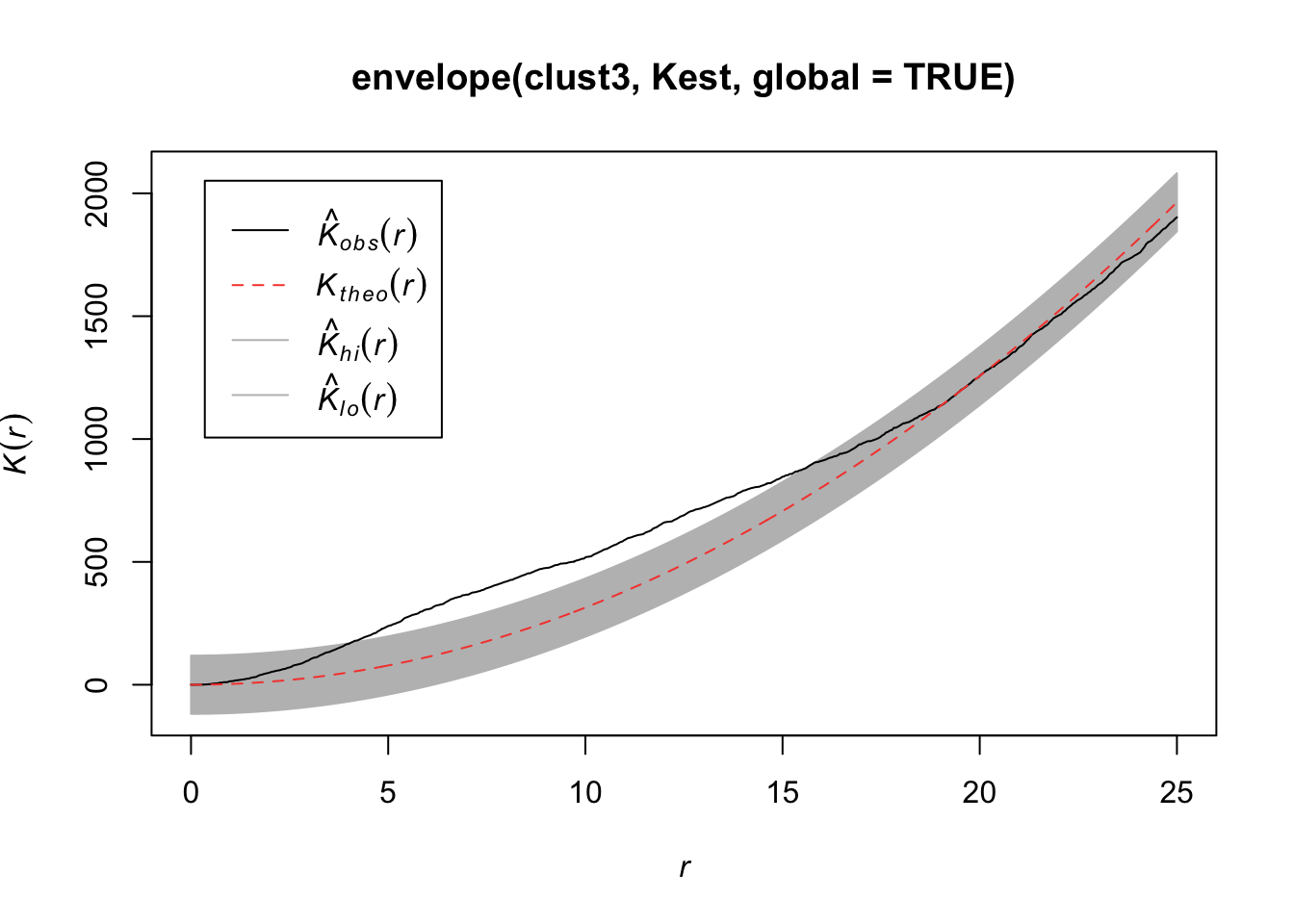

plot(envelope(clust3, Lest, global = TRUE))

## Generating 99 simulations of CSR  ...
## 1, 2, 3, 4, 5, 6, 7, 8, 9, 10, 11, 12, 13, 14, 15, 16, 17, 18, 19, 20, 21, 22, 23, 24, 25, 26, 27, 28, 29, 30, 31, 32, 33, 34, 35,
## 36, 37, 38, 39, 40, 41, 42, 43, 44, 45, 46, 47, 48, 49, 50, 51, 52, 53, 54, 55, 56, 57, 58, 59, 60, 61, 62, 63, 64, 65, 66, 67, 68, 69, 70,
## 71, 72, 73, 74, 75, 76, 77, 78, 79, 80, 81, 82, 83, 84, 85, 86, 87, 88, 89, 90, 91, 92, 93, 94, 95, 96, 97, 98,  99.
## 
## Done.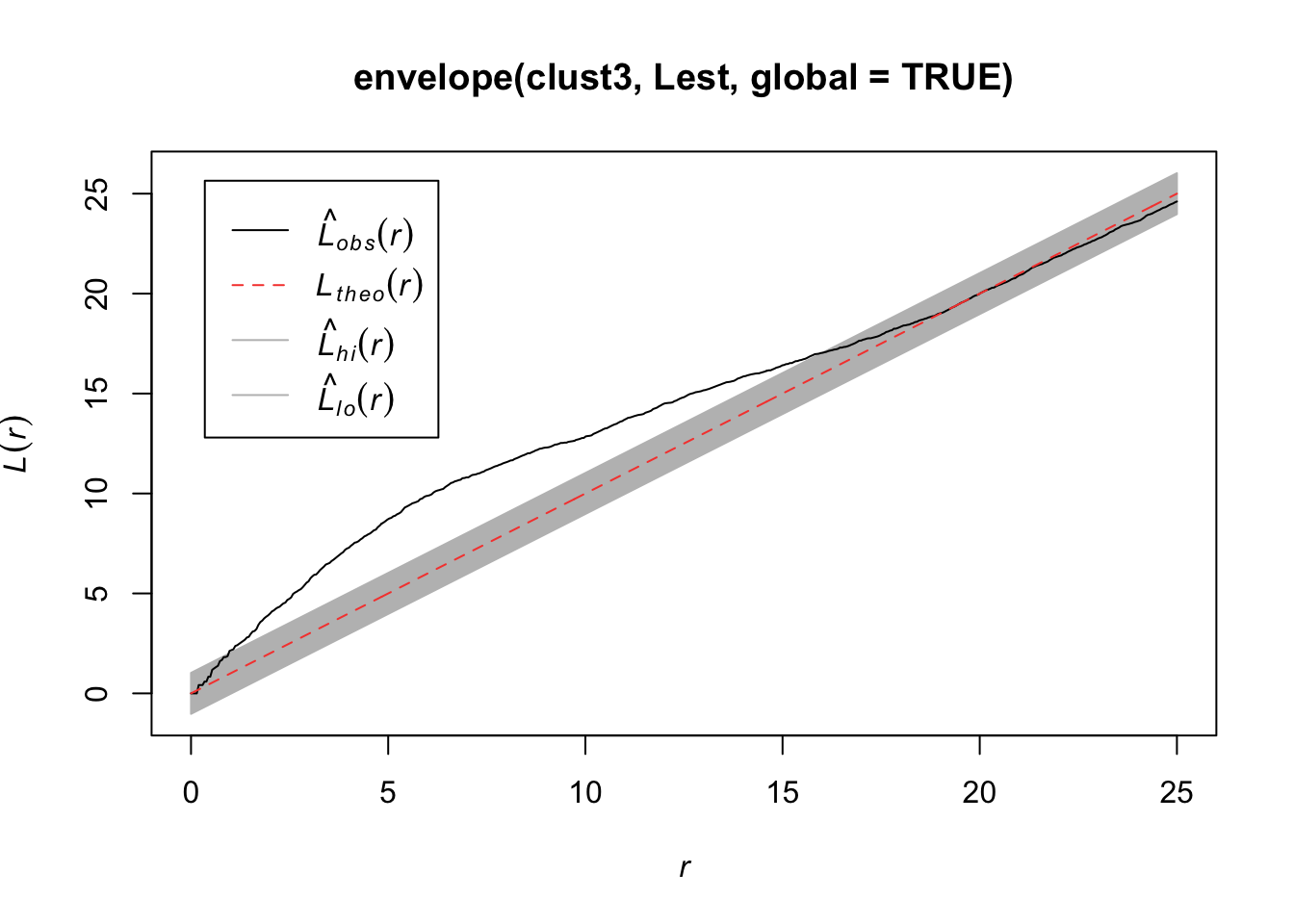

7.2.5.3 Fitting Cluster Poisson Process Models

If you believe the data are clustered, you can fit a model that accounts for any trends in \(\lambda(s)\) as well as clustering in points in the generation process. Two potential models you can fit are the Thomas and the Matern model.

plot(redwood)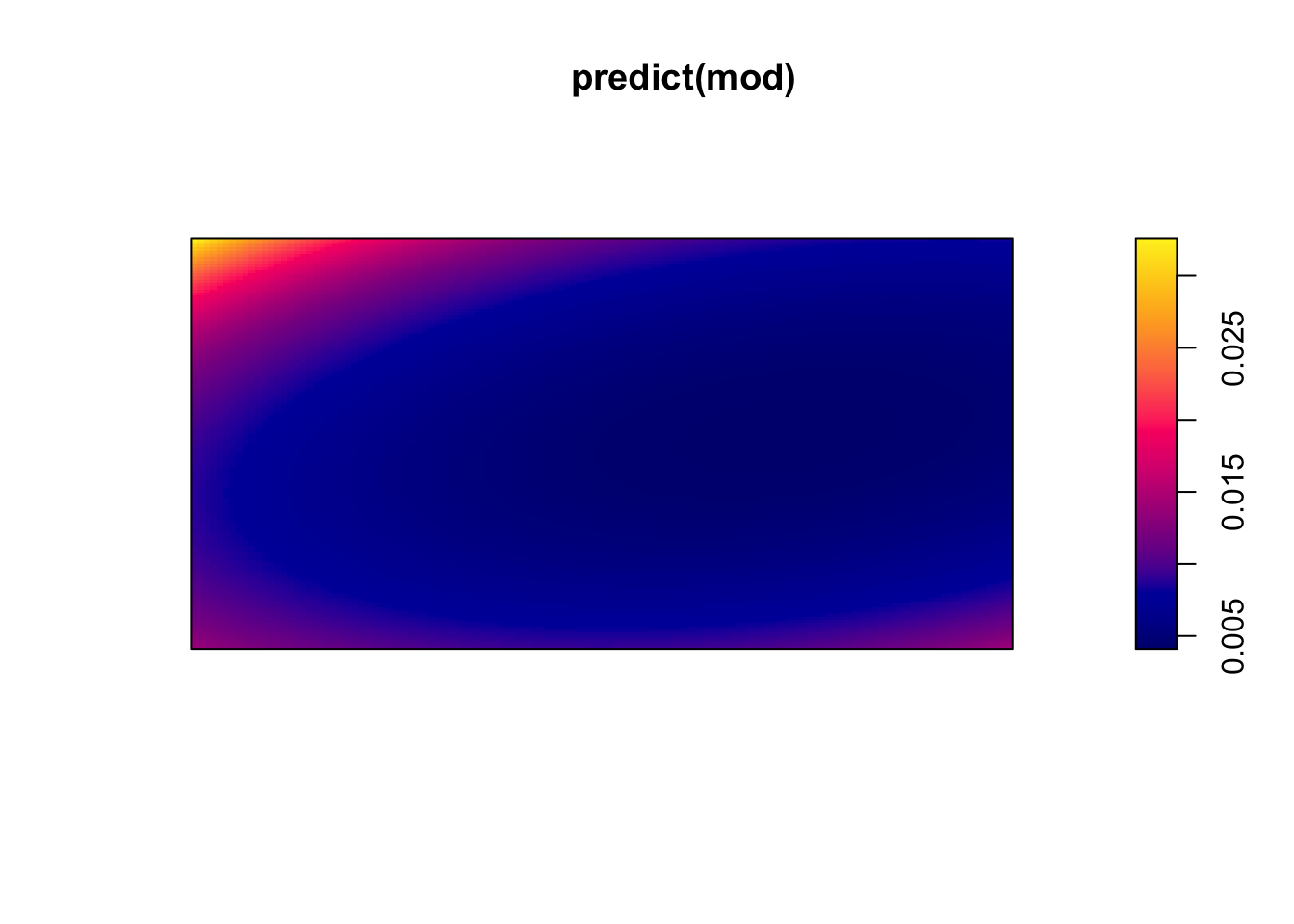

summary(kppm(redwood, ~1, "Thomas"))

## Stationary cluster point process model
## Fitted to point pattern dataset 'redwood'
## Fitted by minimum contrast
##  Summary statistic: K-function
## Minimum contrast fit (object of class "minconfit")
## Model: Thomas process
## Fitted by matching theoretical K function to redwood
## 
## Internal parameters fitted by minimum contrast ($par):
##     kappa    sigma2 
## 23.548568  0.002214 
## 
## Fitted cluster parameters:
##    kappa    scale 
## 23.54857  0.04705 
## Mean cluster size:  2.633 points
## 
## Converged successfully after 105 function evaluations
## 
## Starting values of parameters:
##     kappa    sigma2 
## 62.000000  0.006173 
## Domain of integration: [ 0 , 0.25 ]
## Exponents: p= 2, q= 0.25
## 
## ----------- TREND MODEL -----
## Point process model
## Fitting method: maximum likelihood (Berman-Turner approximation)
## Model was fitted using glm()
## Algorithm converged
## Call:
## ppm.ppp(Q = X, trend = trend, rename.intercept = FALSE, covariates = covariates, 
##     covfunargs = covfunargs, use.gam = use.gam, forcefit = TRUE, 
##     nd = nd, eps = eps)
## Edge correction: "border"
##  [border correction distance r = 0 ]
## ----------------------------------------------------------------------
## Quadrature scheme (Berman-Turner) = data + dummy + weights
## 
## Data pattern:
## Planar point pattern:  62 points
## Average intensity 62 points per square unit
## Window: rectangle = [0, 1] x [-1, 0] units
##                     (1 x 1 units)
## Window area = 1 square unit
## 
## Dummy quadrature points:
##      32 x 32 grid of dummy points, plus 4 corner points
##      dummy spacing: 0.03125 units
## 
## Original dummy parameters: =
## Planar point pattern:  1028 points
## Average intensity 1030 points per square unit
## Window: rectangle = [0, 1] x [-1, 0] units
##                     (1 x 1 units)
## Window area = 1 square unit
## Quadrature weights:
##      (counting weights based on 32 x 32 array of rectangular tiles)
## All weights:
##  range: [0.000326, 0.000977] total: 1
## Weights on data points:
##  range: [0.000326, 0.000488] total: 0.0277
## Weights on dummy points:
##  range: [0.000326, 0.000977] total: 0.972
## ----------------------------------------------------------------------
## FITTED MODEL:
## 
## Stationary Poisson process
## 
## ---- Intensity: ----
## 
## 
## Uniform intensity:
## [1] 62
## 
##             Estimate  S.E. CI95.lo CI95.hi Ztest Zval
## (Intercept)    4.127 0.127   3.878   4.376   *** 32.5
## 
## ----------- gory details -----
## 
## Fitted regular parameters (theta):
## (Intercept) 
##       4.127 
## 
## Fitted exp(theta):
## (Intercept) 
##          62 
## 
## ----------- CLUSTER MODEL -----------
## Model: Thomas process
## 
## Fitted cluster parameters:
##    kappa    scale 
## 23.54857  0.04705 
## Mean cluster size:  2.633 points
## 
## Final standard error and CI
## (allowing for correlation of cluster process):
##             Estimate   S.E. CI95.lo CI95.hi Ztest  Zval
## (Intercept)    4.127 0.2329   3.671   4.584   *** 17.72
## 
## ----------- cluster strength indices ----------
## Sibling probability 0.6042
## Count overdispersion index (on original window): 3.409

AIC(kppm(redwood, ~1, "Thomas", method = "palm"))

## [1] -2478

summary(kppm(redwood, ~x, "Thomas"))

## Inhomogeneous cluster point process model
## Fitted to point pattern dataset 'redwood'
## Fitted by minimum contrast
##  Summary statistic: inhomogeneous K-function
## Minimum contrast fit (object of class "minconfit")
## Model: Thomas process
## Fitted by matching theoretical K function to redwood
## 
## Internal parameters fitted by minimum contrast ($par):
##     kappa    sigma2 
## 22.917939  0.002148 
## 
## Fitted cluster parameters:
##    kappa    scale 
## 22.91794  0.04635 
## Mean cluster size:  [pixel image]
## 
## Converged successfully after 85 function evaluations
## 
## Starting values of parameters:
##     kappa    sigma2 
## 62.000000  0.006173 
## Domain of integration: [ 0 , 0.25 ]
## Exponents: p= 2, q= 0.25
## 
## ----------- TREND MODEL -----
## Point process model
## Fitting method: maximum likelihood (Berman-Turner approximation)
## Model was fitted using glm()
## Algorithm converged
## Call:
## ppm.ppp(Q = X, trend = trend, rename.intercept = FALSE, covariates = covariates, 
##     covfunargs = covfunargs, use.gam = use.gam, forcefit = TRUE, 
##     nd = nd, eps = eps)
## Edge correction: "border"
##  [border correction distance r = 0 ]
## ----------------------------------------------------------------------
## Quadrature scheme (Berman-Turner) = data + dummy + weights
## 
## Data pattern:
## Planar point pattern:  62 points
## Average intensity 62 points per square unit
## Window: rectangle = [0, 1] x [-1, 0] units
##                     (1 x 1 units)
## Window area = 1 square unit
## 
## Dummy quadrature points:
##      32 x 32 grid of dummy points, plus 4 corner points
##      dummy spacing: 0.03125 units
## 
## Original dummy parameters: =
## Planar point pattern:  1028 points
## Average intensity 1030 points per square unit
## Window: rectangle = [0, 1] x [-1, 0] units
##                     (1 x 1 units)
## Window area = 1 square unit
## Quadrature weights:
##      (counting weights based on 32 x 32 array of rectangular tiles)
## All weights:
##  range: [0.000326, 0.000977] total: 1
## Weights on data points:
##  range: [0.000326, 0.000488] total: 0.0277
## Weights on dummy points:
##  range: [0.000326, 0.000977] total: 0.972
## ----------------------------------------------------------------------
## FITTED MODEL:
## 
## Nonstationary Poisson process
## 
## ---- Intensity: ----
## 
## Log intensity: ~x
## 
## Fitted trend coefficients:
## (Intercept)           x 
##      3.9746      0.2977 
## 
##             Estimate   S.E. CI95.lo CI95.hi Ztest    Zval
## (Intercept)   3.9746 0.2640  3.4572   4.492   *** 15.0567
## x             0.2977 0.4409 -0.5665   1.162        0.6751
## 
## ----------- gory details -----
## 
## Fitted regular parameters (theta):
## (Intercept)           x 
##      3.9746      0.2977 
## 
## Fitted exp(theta):
## (Intercept)           x 
##      53.228       1.347 
## 
## ----------- CLUSTER MODEL -----------
## Model: Thomas process
## 
## Fitted cluster parameters:
##    kappa    scale 
## 22.91794  0.04635 
## Mean cluster size:  [pixel image]
## 
## Final standard error and CI
## (allowing for correlation of cluster process):
##             Estimate   S.E. CI95.lo CI95.hi Ztest   Zval
## (Intercept)   3.9746 0.4642   3.065   4.884   *** 8.5626
## x             0.2977 0.7850  -1.241   1.836       0.3792
## 
## ----------- cluster strength indices ----------
## Mean sibling probability 0.6178
## Count overdispersion index (on original window): 3.494

AIC(kppm(redwood, ~x, "Thomas", method = "palm"))

## [1] -2465

summary(kppm(redwood, ~1, "MatClust"))

## Stationary cluster point process model
## Fitted to point pattern dataset 'redwood'
## Fitted by minimum contrast
##  Summary statistic: K-function
## Minimum contrast fit (object of class "minconfit")
## Model: Matern cluster process
## Fitted by matching theoretical K function to redwood
## 
## Internal parameters fitted by minimum contrast ($par):
##    kappa        R 
## 24.55865  0.08654 
## 
## Fitted cluster parameters:
##    kappa    scale 
## 24.55865  0.08654 
## Mean cluster size:  2.525 points
## 
## Converged successfully after 57 function evaluations
## 
## Starting values of parameters:
##    kappa        R 
## 62.00000  0.07857 
## Domain of integration: [ 0 , 0.25 ]
## Exponents: p= 2, q= 0.25
## 
## ----------- TREND MODEL -----
## Point process model
## Fitting method: maximum likelihood (Berman-Turner approximation)
## Model was fitted using glm()
## Algorithm converged
## Call:
## ppm.ppp(Q = X, trend = trend, rename.intercept = FALSE, covariates = covariates, 
##     covfunargs = covfunargs, use.gam = use.gam, forcefit = TRUE, 
##     nd = nd, eps = eps)
## Edge correction: "border"
##  [border correction distance r = 0 ]
## ----------------------------------------------------------------------
## Quadrature scheme (Berman-Turner) = data + dummy + weights
## 
## Data pattern:
## Planar point pattern:  62 points
## Average intensity 62 points per square unit
## Window: rectangle = [0, 1] x [-1, 0] units
##                     (1 x 1 units)
## Window area = 1 square unit
## 
## Dummy quadrature points:
##      32 x 32 grid of dummy points, plus 4 corner points
##      dummy spacing: 0.03125 units
## 
## Original dummy parameters: =
## Planar point pattern:  1028 points
## Average intensity 1030 points per square unit
## Window: rectangle = [0, 1] x [-1, 0] units
##                     (1 x 1 units)
## Window area = 1 square unit
## Quadrature weights:
##      (counting weights based on 32 x 32 array of rectangular tiles)
## All weights:
##  range: [0.000326, 0.000977] total: 1
## Weights on data points:
##  range: [0.000326, 0.000488] total: 0.0277
## Weights on dummy points:
##  range: [0.000326, 0.000977] total: 0.972
## ----------------------------------------------------------------------
## FITTED MODEL:
## 
## Stationary Poisson process
## 
## ---- Intensity: ----
## 
## 
## Uniform intensity:
## [1] 62
## 
##             Estimate  S.E. CI95.lo CI95.hi Ztest Zval
## (Intercept)    4.127 0.127   3.878   4.376   *** 32.5
## 
## ----------- gory details -----
## 
## Fitted regular parameters (theta):
## (Intercept) 
##       4.127 
## 
## Fitted exp(theta):
## (Intercept) 
##          62 
## 
## ----------- CLUSTER MODEL -----------
## Model: Matern cluster process
## 
## Fitted cluster parameters:
##    kappa    scale 
## 24.55865  0.08654 
## Mean cluster size:  2.525 points
## 
## Final standard error and CI
## (allowing for correlation of cluster process):
##             Estimate   S.E. CI95.lo CI95.hi Ztest  Zval
## (Intercept)    4.127 0.2303   3.676   4.579   *** 17.92
## 
## ----------- cluster strength indices ----------
## Sibling probability 0.6338
## Count overdispersion index (on original window): 3.326

AIC(kppm(redwood, ~1, "MatClust", method = "palm"))

## [1] -2476

summary(kppm(redwood, ~x, "MatClust"))

## Inhomogeneous cluster point process model
## Fitted to point pattern dataset 'redwood'
## Fitted by minimum contrast
##  Summary statistic: inhomogeneous K-function
## Minimum contrast fit (object of class "minconfit")
## Model: Matern cluster process
## Fitted by matching theoretical K function to redwood
## 
## Internal parameters fitted by minimum contrast ($par):
##    kappa        R 
## 23.89160  0.08524 
## 
## Fitted cluster parameters:
##    kappa    scale 
## 23.89160  0.08524 
## Mean cluster size:  [pixel image]
## 
## Converged successfully after 55 function evaluations
## 
## Starting values of parameters:
##    kappa        R 
## 62.00000  0.07857 
## Domain of integration: [ 0 , 0.25 ]
## Exponents: p= 2, q= 0.25
## 
## ----------- TREND MODEL -----
## Point process model
## Fitting method: maximum likelihood (Berman-Turner approximation)
## Model was fitted using glm()
## Algorithm converged
## Call:
## ppm.ppp(Q = X, trend = trend, rename.intercept = FALSE, covariates = covariates, 
##     covfunargs = covfunargs, use.gam = use.gam, forcefit = TRUE, 
##     nd = nd, eps = eps)
## Edge correction: "border"
##  [border correction distance r = 0 ]
## ----------------------------------------------------------------------
## Quadrature scheme (Berman-Turner) = data + dummy + weights
## 
## Data pattern:
## Planar point pattern:  62 points
## Average intensity 62 points per square unit
## Window: rectangle = [0, 1] x [-1, 0] units
##                     (1 x 1 units)
## Window area = 1 square unit
## 
## Dummy quadrature points:
##      32 x 32 grid of dummy points, plus 4 corner points
##      dummy spacing: 0.03125 units
## 
## Original dummy parameters: =
## Planar point pattern:  1028 points
## Average intensity 1030 points per square unit
## Window: rectangle = [0, 1] x [-1, 0] units
##                     (1 x 1 units)
## Window area = 1 square unit
## Quadrature weights:
##      (counting weights based on 32 x 32 array of rectangular tiles)
## All weights:
##  range: [0.000326, 0.000977] total: 1
## Weights on data points:
##  range: [0.000326, 0.000488] total: 0.0277
## Weights on dummy points:
##  range: [0.000326, 0.000977] total: 0.972
## ----------------------------------------------------------------------
## FITTED MODEL:
## 
## Nonstationary Poisson process
## 
## ---- Intensity: ----
## 
## Log intensity: ~x
## 
## Fitted trend coefficients:
## (Intercept)           x 
##      3.9746      0.2977 
## 
##             Estimate   S.E. CI95.lo CI95.hi Ztest    Zval
## (Intercept)   3.9746 0.2640  3.4572   4.492   *** 15.0567
## x             0.2977 0.4409 -0.5665   1.162        0.6751
## 
## ----------- gory details -----
## 
## Fitted regular parameters (theta):
## (Intercept)           x 
##      3.9746      0.2977 
## 
## Fitted exp(theta):
## (Intercept)           x 
##      53.228       1.347 
## 
## ----------- CLUSTER MODEL -----------
## Model: Matern cluster process
## 
## Fitted cluster parameters:
##    kappa    scale 
## 23.89160  0.08524 
## Mean cluster size:  [pixel image]
## 
## Final standard error and CI
## (allowing for correlation of cluster process):
##             Estimate   S.E. CI95.lo CI95.hi Ztest   Zval
## (Intercept)   3.9746 0.4599   3.073   4.876   *** 8.6415
## x             0.2977 0.7784  -1.228   1.823       0.3825
## 
## ----------- cluster strength indices ----------
## Mean sibling probability 0.6471
## Count overdispersion index (on original window): 3.41

AIC(kppm(redwood, ~x, "MatClust", method = "palm"))

## [1] -2463

We can then interpret the estimates for that process to tell us about the clustering.

INTERPRETATIONS

theta: parameters for intensity trend
kappa: average number of clusters per unit area
scale: standard deviation of distance of a point from its cluster centre.
mu: mean number of points per cluster

7.2.6 Inhibition Poisson Processes

If points “repel” each other, then we need to account for that as well.

7.2.6.1 Simple Sequential Inhibition

Each new point is generated uniformly in the window (space of interest) and independently of preceding points. If the new point lies closer than r units from an existing point, then it is rejected and another random point is generated. The process terminates when no further points can be added.

plot(rSSI(r = 0.05, n = 200))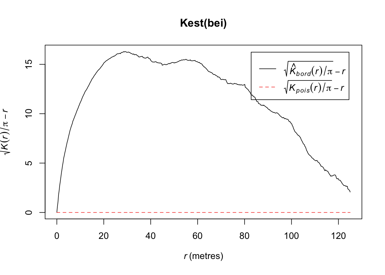

7.2.6.2 Matern I Inhibition Model

In Matern’s Model I, a homogeneous Poisson process Y is first generated (intensity = \(\rho\)). Any pairs of points that lies closer than a distance \(r\) from each other is deleted. Thus, pairs of close neighbours annihilate each other.

The probability an arbitrary point survives is \(e^{-\pi\rho r^2}\) so the intensity of the final point pattern is \(\lambda = \rho e^{-\pi\rho r^2}\).

7.2.7 Other Point Process Models

Markov Point Processes: a large class of models that allow for interaction between points (attraction or repulsion)
Hard Core Gibbs Point Processes: a subclass of Markov Point Processes that allows for interaction between points; no interaction is a Poisson point process
Strauss Processes: a subclass of Markov Point Processes that allow for repulsion between pairs of points
Cox Processes: a doubly stochastic Poisson process in which the intensity is a random process and conditional on the intensity, the events are an inhomogenous Poisson process.

For more information on how to fit spatial point processes in R, see http://www3.uji.es/~mateu/badturn.pdf.