7.4 Point Referenced Data
A spatial stochastic process is a spatially indexed collection of random variables,
\[\{Y(s): s\in D \subset \mathbb{R}^d \}\]
where \(d\) will typically be 2 or 3.
A realization from a stochastic process is sometimes referred to as a sample path. We typically observe a vector
\[Y \equiv Y(s_1),...,Y(s_n)\]
7.4.1 Gaussian Process
A Gaussian process (GP) has finite-dimensional distributions that are all multivariate normal and we define it using a mean and coviariance function,
\[\mu(s) = E(Y(s))\] \[C(s_1,s_2) = Cov(Y(s_1),Y(s_2))\]
As with time series and longitudinal data, we must consider the covariance of our data. Most covariance models that we will consider in this course require that our data came from a statitionary, isotropic process such that the mean is constant across space, variance is constant across space and the covariance is only a function of the distance between locations (disregarding the direction) such that
\[ E(Y(s)) = E(Y(s+h)) = \mu\] \[Cov(Y(s),Y(s+h)) = Cov(Y(0),Y(h)) = C(||h||)\]
7.4.2 Covariance Models
A covariance model that is often used in spatial data is called the Matern class of covariance functions,
\[C(t) = \frac{\sigma^2}{2^{\nu-1}\Gamma(\nu)}(t\rho)^\nu \mathcal{K}_\nu(d/\rho)\]
where \(\mathcal{K}_\nu\) is a modified Bessel function of order \(\nu\). \(\nu\) is a smoothness parameter and if we let \(\nu = 1/2\), we get the exponential covariance.
7.4.3 Variograms, Semivariograms
Beyond the standard definition of stationarity, there is another form of stationary (intrinsic stationarity), which is when
\[Var(Y(s+h) - Y(s))\text{ depends only on h}\]
When this is true, we call
\[\gamma(h) = \frac{1}{2}Var(Y(s+h) - Y(s))\]
the semivariogram and \(2\gamma(h)\) the variogram.
In fact, if a covariance function is stationary, it will be intrinsic stationary and
\[\gamma(h) = C(0) - C(h) = C(0) (1-\rho(h))\] where \(C(0)\) is the variance (referred to as the sill).
To estimate the semivariogram, first fit a trend so that you have a stationary process in your residuals.
- Let \(H_1,...,H_k\) be a partition of the space of possible lags, with \(h_u\) being a representative spatial lag/distance in \(H_u\). Then use your residuals to estimate the empirical semivariagram.
\[\hat{\gamma}(h_u) = \frac{1}{2\cdot |\{s_i-s_j \in H_u\}|}\sum_{\{s_i-s_j\in H_u\}}(e(s_i) - e(s_j))^2\]
- This is a non-parametric estimate of the semivariogram.
library(gstat)
coordinates(meuse) = ~x + y

estimatedVar <- variogram(log(zinc) ~ 1, data = meuse)
plot(estimatedVar)
- If we notice a particular pattern in the points, we could try and fit a curve based on models for correlation.
Var.fit1 <- fit.variogram(estimatedVar, model = vgm(1, "Sph", 900, 1))
plot(estimatedVar, Var.fit1)
Var.fit1## model psill range
## 1 Nug 0.05066 0
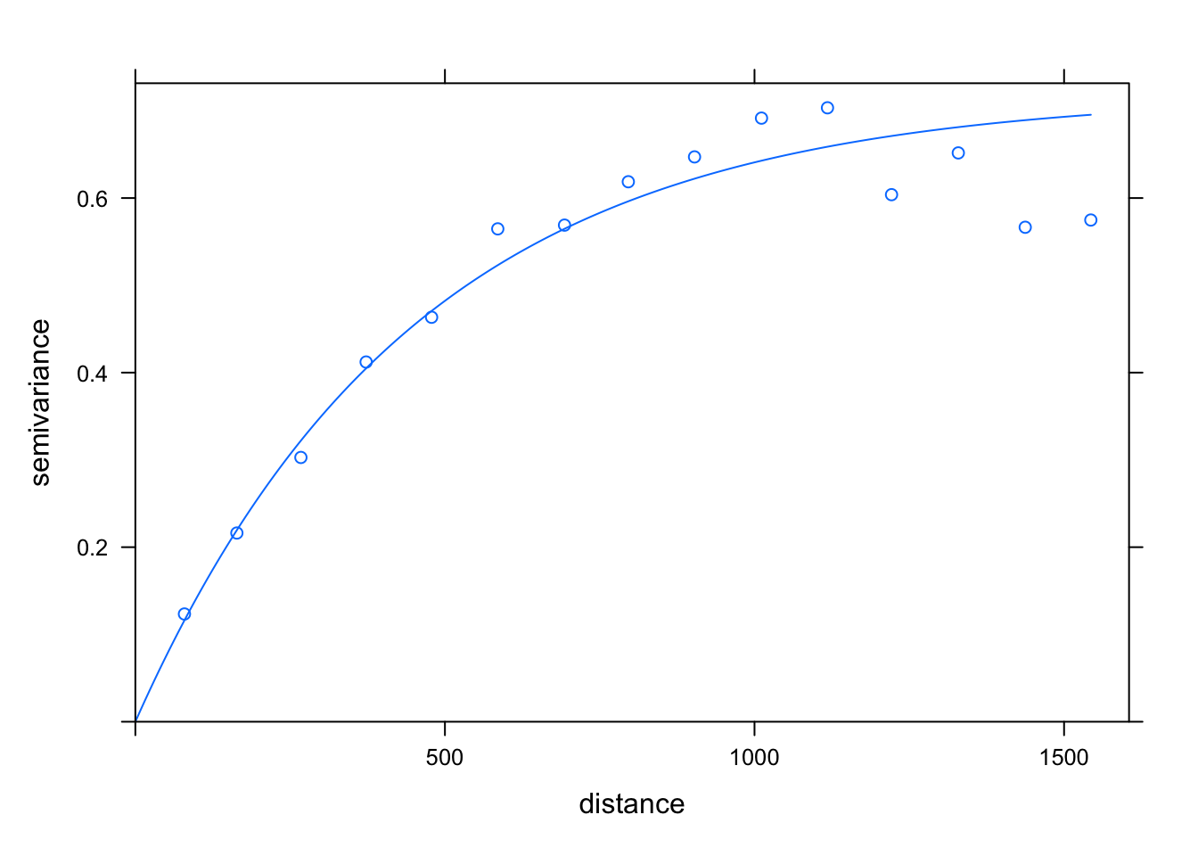
## 2 Sph 0.59061 897Var.fit2 <- fit.variogram(estimatedVar, model = vgm(1, "Exp", 900, 1))
plot(estimatedVar, Var.fit2)
Var.fit3 <- fit.variogram(estimatedVar, model = vgm(1, "Gau", 900, 1))
plot(estimatedVar, Var.fit3)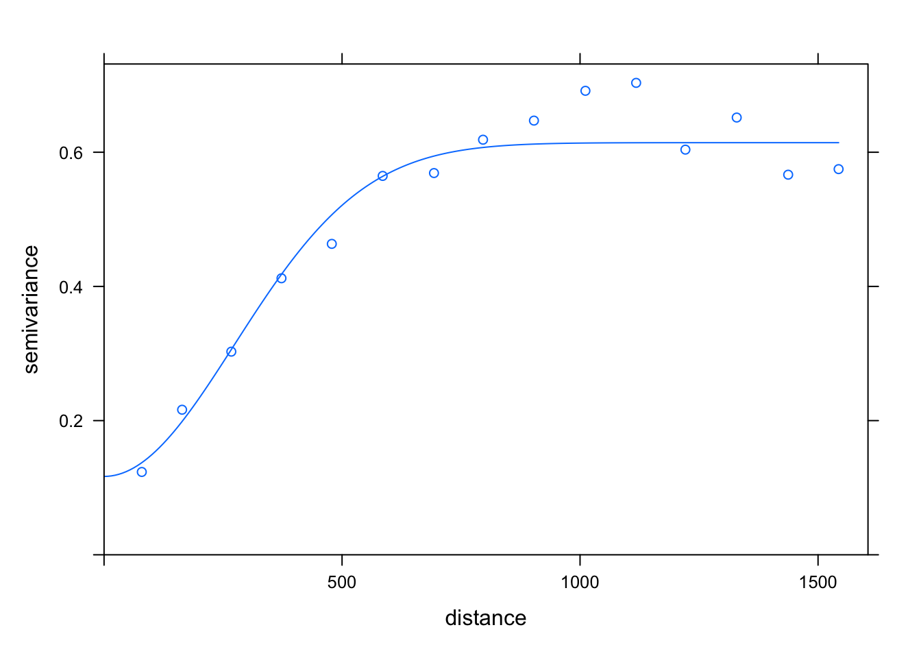
Var.fit4 <- fit.variogram(estimatedVar, model = vgm(1, "Mat", 900, 1))
plot(estimatedVar, Var.fit4)