Spatial Data

Coordinate Reference System

At the heart of every spatial data is a set of locations. One way to describe a location is in terms of coordinates and a coordinate reference system (CRS).

There are three main components to a CRS: ellipsoid, datum, and a projection. (The projection is a part of a projected CRS.)

Ellipsoid

The Earth is not a sphere.
- It’s closer to a bumpy ellipsoid with a bulge at the equator.
The ellipsoid part of a CRS is a mathematical model giving a smooth approximation to Earth’s shape.
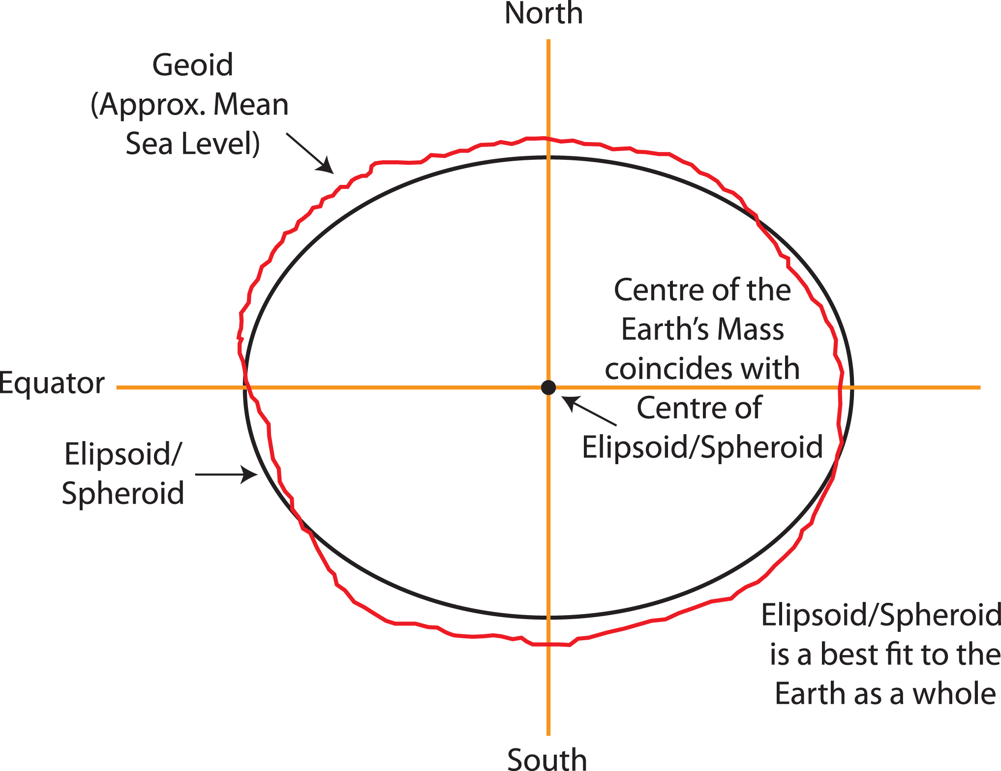
Common ellipsoid models: WGS84 and GRS80

Datum

Where do we center the ellipsoid? This center is called a datum.
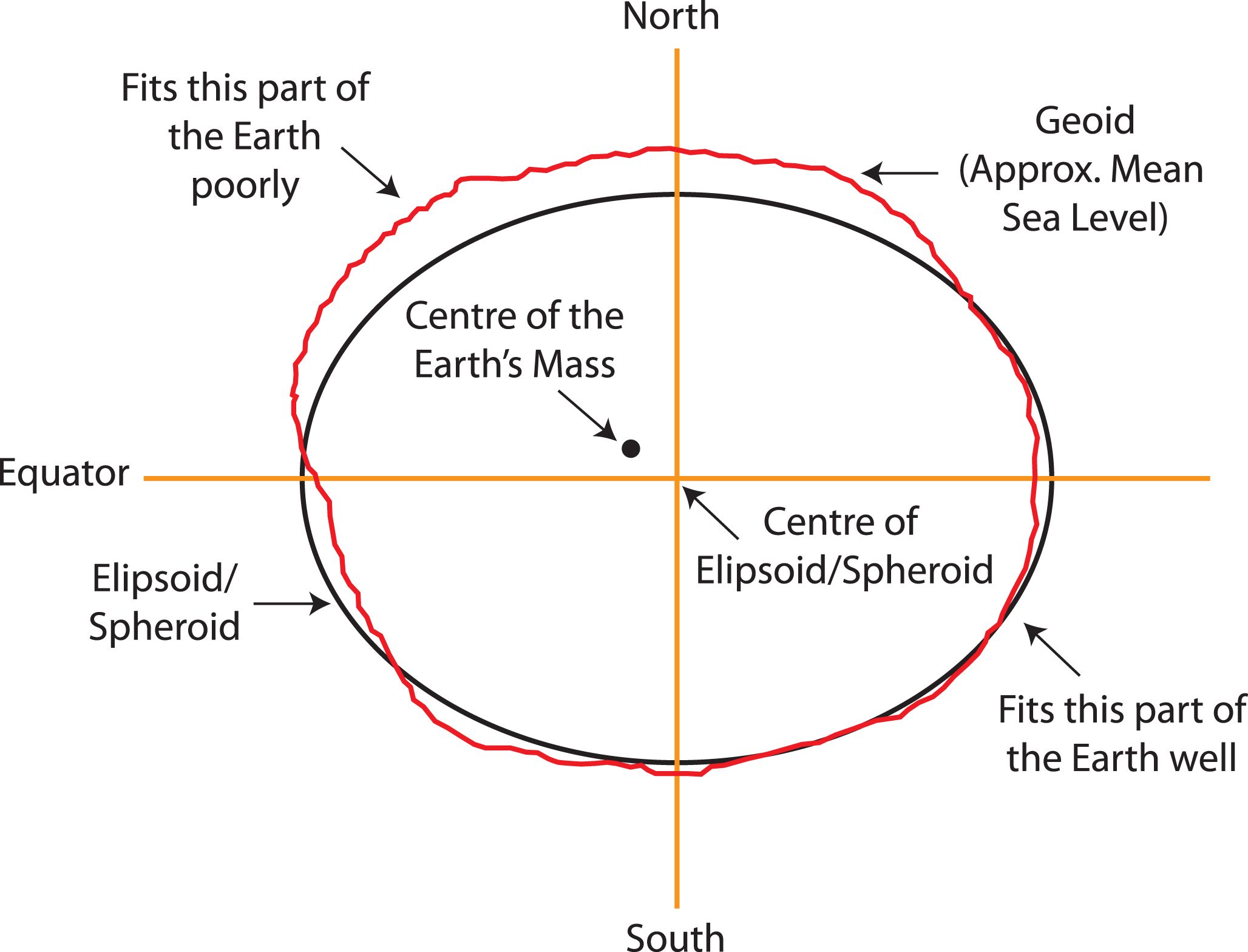
For a given ellipsoid model, different datums are used to better fit different areas of the world.
- e.g., For the GRS80 ellipsoid, the NAD83 datum is a good fit in North America, but SIRGAS2000 is a better fit in South America.
- The Global Positioning System (GPS) uses the WGS84 ellipsoid model and WGS84 datum. This provides an overall best fit of the Earth.

Why do the ellipsoid and datum matter?

If you have longitude and latitude coordinates for a location, you need to know what datum and ellipsoid were used to define those positions in order to overlay those points correctly on a map.

Note: In practice, the horizontal distance between WGS84 and NAD83 coordinates is about 3-4 feet in the US, which may not be significant for most applications.

Projection

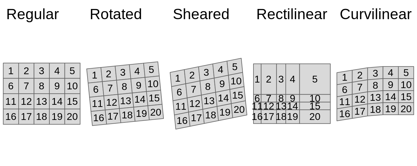
Lastly, the Earth lives in a 3 dimensional (3D) world and most visualizations are on a 2 dimensional (2D) surface. We must choose a projection method to represent points, regions, and lines on Earth on a 2D map with distance units (typically meter, international foot, US survey foot). In that projection process, a 3D element will lose angle, area, and/or distance when projected onto a 2D surface, no matter which method is chosen.

For a good overview of common projection methods, see https://pubs.usgs.gov/gip/70047422/report.pdf.
Common projection: Mercator projection
- Cylindrical map projection from the 1500’s
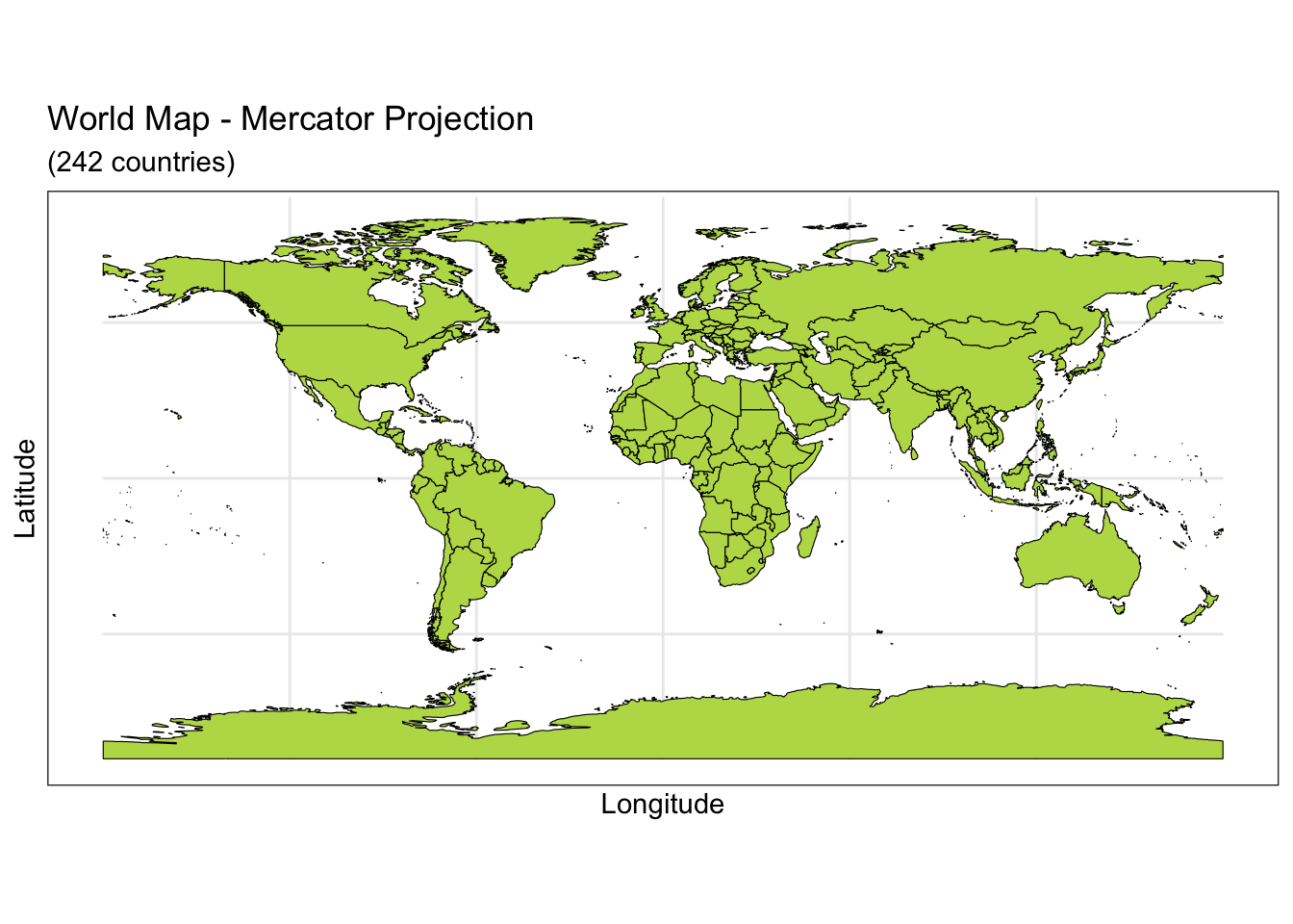
- Useful for navigation because it represented north as up and south as down everywhere and preserves local directions and shape
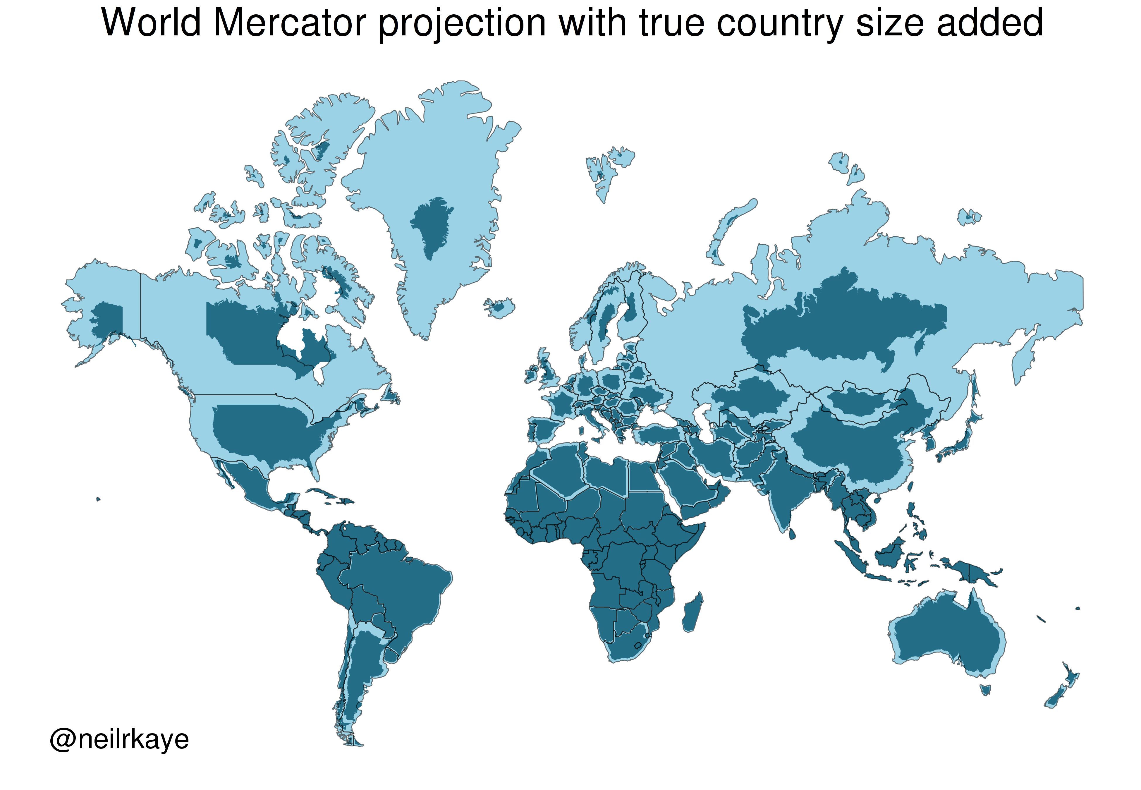
- Drawback: it inflates the size of regions far from the equator. Greenland, Antarctica, Canada, and Russia appear much bigger than they should. The illustration below compares country areas/shapes under the Mercator projection (light blue) with true areas/shapes (dark blue).

Below you can see four different world projections. Take note of what is lost in terms of angle, area, or distance in these projections.

library(tidyverse)
library(sf)
world <- rnaturalearth::ne_countries(scale = "medium", returnclass = "sf")

# Basic Map w/ labels
ggplot(data = world) + 
    geom_sf(color = "black", fill = "#bada55") +
    labs(x = "Longitude", y = "Latitude", title = "World Map - Mercator Projection", subtitle = paste0("(", length(unique(world$name)), " countries)")) +
    theme_bw()

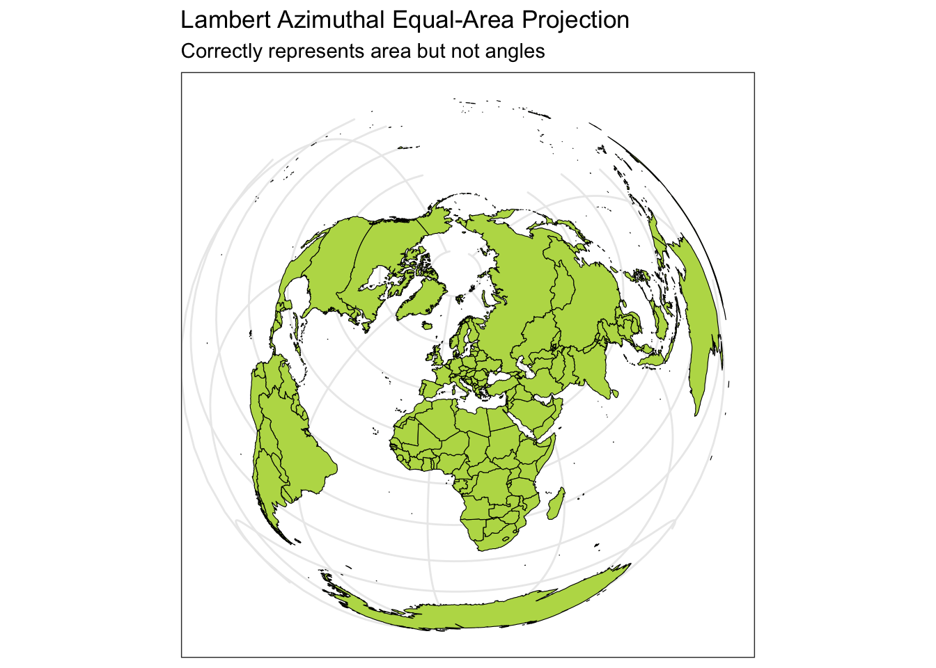
ggplot(data = world) +
    geom_sf(color = "black", fill = "#bada55") +
    coord_sf(crs = "+proj=laea +lat_0=52 +lon_0=10 +x_0=4321000 +y_0=3210000 +ellps=GRS80 +units=m +no_defs") + 
    labs(title = "Lambert Azimuthal Equal-Area Projection", subtitle = "Correctly represents area but not angles") + 
    theme_bw()

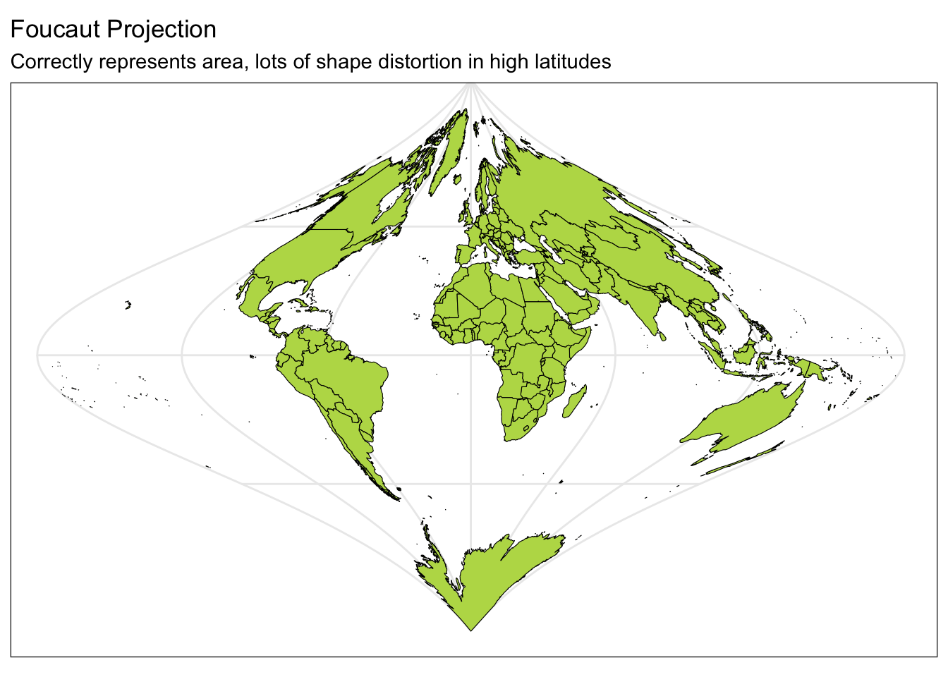
ggplot(data = world) +
    geom_sf(color = "black", fill = "#bada55") +
    coord_sf(crs = "+proj=fouc") + 
    labs(title = "Foucaut Projection", subtitle = "Correctly represents area, lots of shape distortion in high latitudes") + 
    theme_bw()

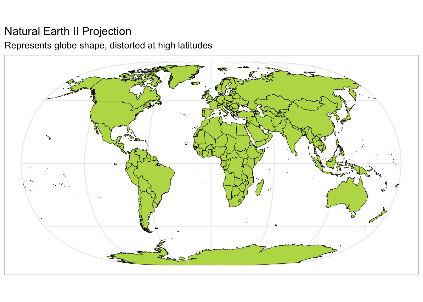
ggplot(data = world) +
    geom_sf(color = "black", fill = "#bada55") +
    coord_sf(crs = "+proj=natearth2") + 
    labs(title = "Natural Earth II Projection", subtitle = "Represents globe shape, distorted at high latitudes") + 
    theme_bw()

Spatial data

With a CRS to collect and record location data in terms of longitude or easting (x) and latitude or northing (y) coordinates, we can now consider common models for storing spatial data on the computer. There are two main data models: vector and raster.

Vector

Vector data represents the world as a set of spatial geometries that are defined in terms of location coordinates (with a specified CRS) with non-spatial attributes or properties.

The three basic vector geometries are:

Points: Locations defined based on a (x, y) coordinates.
- e.g., Cities
Lines: A set of ordered points connected by straight lines.
- e.g., Roads, rivers
Polygons: A set of ordered points connected by straight lines, first and last point are the same.
- e.g., Geopolitical boundaries, bodies of water

File formats:

Text files (e.g., .csv)
- x and y columns: for coordinates (x for longitude and y for latitude)
- group id column: needed for lines and polygons
- additional columns: attributes related to the areas in each row (e.g., population sizes, demographic information)
- Text files do not store the CRS.
Shapefiles (.shp)
- Widely supported spatial vector file format (that includes the CRS).
GeoJSON (.geojson) (Geographical Javascript Object Notation)
KML (.kml) (Keyhole Markup Language)

Raster

Continuous grid of cells where each cell has a single value.
- Continuous values (e.g., elevation, precipitation)
- Categorical values (e.g., land cover type, soil type)
Shape of cells
- Generally square (like pixels)
- Cells can be rotated and sheared. Rectilinear and curvilinear shapes are also possible, depending on the spatial region of interest and CRS.

Computational time considerations

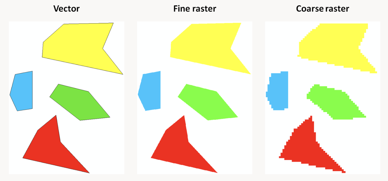
High resolution raster data involves a large number of small cells. This results in large file sizes and objects which can make computation and visualization quite slow.

File formats:

GeoTIFF (.tif or .tiff)
- Most popular
NetCDF (.nc)
HDF (.hdf)

To work with raster data in R, you’ll use the raster, terra, and the stars packages. If you are interested in learning more, check out https://r-spatial.github.io/stars/.