Topic 12 Evaluating Classification Models
Learning Goals
- Calculate (by hand from confusion matrices) and contextually interpret overall accuracy, sensitivity, and specificity
- Construct and interpret plots of predicted probabilities across classes
- Explain how a ROC curve is constructed and the rationale behind AUC as an evaluation metric
- Appropriately use and interpret the no-information rate to evaluate accuracy metrics
Notes: Classification Evaluation
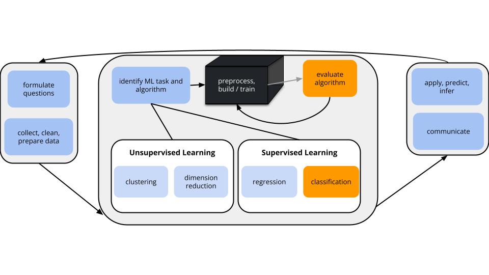
CONTEXT
world = supervised learning
We want to model some output variable \(y\) using a set of potential predictors (\(x_1, x_2, ..., x_p\)).task = CLASSIFICATION
\(y\) is categorical and binary(parametric) algorithm
logistic regressionapplication = classification
- Use our algorithm to calculate the probability that y = 1.
- Turn these into binary classifications using a classification rule. For some probability threshold c:
- If the probability that y = 1 is at least c, classify y as 1.
- Otherwise, classify y as 0.
- WE get to pick c. This should be guided by context (what are the consequences of misclassification?) and the quality of the resulting classifications.
GOAL
Evaluate the quality of binary classifications of \(y\) (here resulting logistic regression model).
Sensitivity & specificity
\[\begin{split} \text{overall accuracy} & = \text{probability of making a correct classification} \\ \text{sensitivity} & = \text{true positive rate}\\ & = \text{probability of correctly classifying $y=1$ as $y=1$} \\ \text{specificity} & = \text{true negative rate} \\ & = \text{probability of correctly classifying $y=0$ as $y=0$} \\ \text{1 - specificity} & = \text{false positive rate} \\ & = \text{probability of classifying $y=0$ as $y=1$} \\ \end{split}\]
In-sample estimation (how well our model classifies the same data points we used to build it)
| y = 0 | y = 1 | |
|---|---|---|
| classify as 0 | a | b |
| classify as 1 | c | d |
\[\begin{split} \text{overall accuracy} & = \frac{a + d}{a + b + c + d}\\ \text{sensitivity} & = \frac{d}{b + d} \\ \text{specificity} & = \frac{a}{a + c} \\ \end{split}\]
k-Fold Cross-Validation (how well our model classifies NEW data points)
- Divide the data into k folds of approximately equal size.
- Repeat the following procedures for each fold j = 1, 2, …, k:
- Remove fold j from the data set.
- Fit a model using the other k - 1 folds.
- Use this model to classify the outcomes for the data points in fold j.
- Calculate the overall accuracy, sensitivity, and specificity of these classifications.
- Remove fold j from the data set.
- Average the metrics across the k folds. This gives our CV estimates of overall accuracy, sensitivity, and specificity.
ROC curves (receiver operating characteristic curves)
Sensitivity and specificity depend upon the specific probability threshold c.
If we lower c, hence make it easier to classify y as 1: sensitivity increases but specificity decreases
If we increase c, hence make it tougher to classify y as 1: specificity increases but sensitivity decreases
To understand this trade-off, for a range of possible thresholds c between 0 and 1, ROC curves calculate and plot
- y-axis: sensitivity (true positive rate)
- x-axis: 1 - specificity (false positive rate)
Since specificity is the probability of classifying y = 0 as 0, 1 - specificity is the misclassifying y = 0 as 1.
Why we care:
- Along with context, ROC curves can help us identify an appropriate probability threshold c.
- ROC curves can help us compare the quality of different models.
- The area under an ROC curve (AUC) estimates the probability that our algorithm is more likely to classify y = 1 as 1 than to classify y = 0 as 1, hence distinguish between the 2 classes. Put another way: if we give our model 2 data points, one with y = 0 and the other with y = 1, AUC is the probability that we correctly identify which is which.
Small Group Discussion
EXAMPLE 1
Suppose we model RainTomorrow in Sydney using only the number of hours of bright Sunshine today.
Using a probability threshold of 0.5, this model produces the following classification rule:
- If
Sunshine< 3.125, predict rain. - Otherwise, predict no rain.
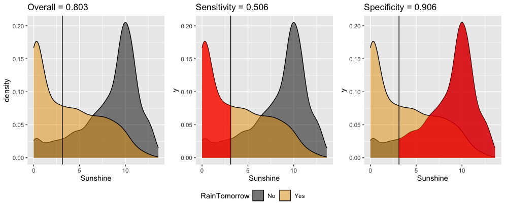
Interpret these in-sample estimates of the resulting classification quality.
- Overall accuracy = 0.803
- We correctly predict the rain outcome (yes or no) 80.3% of the time.
- We correctly predict “no rain” on 80.3% of non-rainy days.
- We correctly predict “rain” on 80.3% of rainy days.
- Sensitivity = 0.506
- We correctly predict the rain outcome (yes or no) 50.6% of the time.
- We correctly predict “no rain” on 50.6% of non-rainy days.
- We correctly predict “rain” on 50.6% of rainy days.
- Specificity = 0.906
- We correctly predict the rain outcome (yes or no) 90.6% of the time.
- We correctly predict “no rain” on 90.6% of non-rainy days.
- We correctly predict “rain” on 90.6% of rainy days.
Solution:
- Overall accuracy = 0.803; We correctly predict the rain outcome (yes or no) 80.3% of the time.
- Sensitivity = 0.506; We correctly predict “rain” on 50.6% of rainy days.
- Specificity = 0.906; We correctly predict “no rain” on 90.6% of non-rainy days.
OPTIONAL EXTRA PRACTICE
Confirm the 3 metrics above using the confusion matrix. Work is shown below (peek when you’re ready).
Solution:
EXAMPLE 2: ROC curves
We can change up the probability threshold in our classification rule!
The ROC curve for our logistic regression model of RainTomorrow by Sunshine plots the sensitivity (true positive rate) vs 1 - specificity (false positive rate) corresponding to “every” possible threshold:
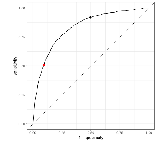
Which point represents the quality of our classification rule using a 0.5 probability threshold?
The other point corresponds to a different classification rule which uses a different threshold. Is that threshold smaller or bigger than 0.5?
Which classification rule do you prefer?
Solution:
- Red point: 0.5 probability rule (sensitivity ~ 0.5, specificity ~ 0.9)
- Black point (higher sensitivity, lower specificity) has a threshold that is lower than 0.5.
- Answers will vary. If you don’t like getting wet (accurately predict rain when it does rain), you’ll want a higher sensitivity. If you don’t like carrying an umbrella when it isn’t needed, you’ll want a higher specificity (lower false positive rate).
EXAMPLE 3: Area Under the ROC Curve (AUC)
The area under an ROC curve (AUC) estimates the probability that our algorithm is more likely to classify y = 1 (rain) as 1 (rain) than to classify y = 0 (no rain) as 1 (rain), hence distinguish between the 2 classes.
AUC is helpful for evaluating and comparing the overall quality of classification models. Consider 3 different possible predictors (A, B, C) of rainy and non-rainy days:
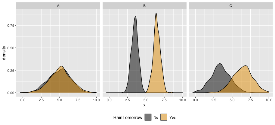
The ROC curves corresponding to the models RainTomorrow ~ A, RainTomorrow ~ B, RainTomorrow ~ C are shown below.
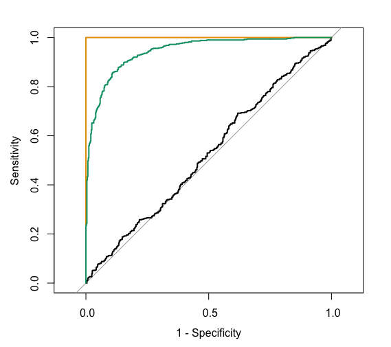
For each ROC curve, indicate the corresponding model and the approximate AUC. Do this in any order you want!
black ROC curve
RainTomorrow ~ ___- AUC is roughly ___
green ROC curve
RainTomorrow ~ ___- AUC is roughly ___.
orange ROC curve
RainTomorrow ~ ___- AUC is exactly ___.
Solution:
black ROC curve
RainTomorrow ~ A- AUC is roughly 0.5
green ROC curve
RainTomorrow ~ C- AUC is roughly .95.
orange ROC curve
RainTomorrow ~ B- AUC is exactly 1.
AUC OBSERVATION
In general:
- A perfect classification model has an AUC of 1.
- The simplest classification model that just randomly predicts y to be 1 or 0 (eg: by flipping a coin), has an AUC of 0.5. It is represented by the diagonal “no discrimination line” in an ROC plot.
- A model with an AUC below 0.5 is worse than just random. Flipping a coin would be better.
Exercises
Today’s in-class exercises will be due as Homework 5.
Please find the exercises and template in Moodle.
I recommend working on Exercises 1, 5, and 6 in class.
Exercise 1 is necessary to the other exercises, and Exercises 5 and 6 involve new content: ROC curves, AUC, and LASSO for classification!
Notes: R code
Let my_model be a logistic regression model of categorical response variable y using predictors x1 and x2 in our sample_data.
# Load packages
library(tidymodels)

# Resolves package conflicts by preferring tidymodels functions
tidymodels_prefer()
# Calculate the probability that y = 1 for each sample data point
# The probability is stored in the .pred_Yes column
in_sample_predictions <- my_model %>%
augment(new_data = sample_data)# Plot the predicted probability that y = 1 by the actual y category
ggplot(in_sample_predictions, aes(y = .pred_Yes, x = y)) +
geom_boxplot()# Calculate sensitivity & specificity for a range of probability thresholds
in_sample_predictions %>%
roc_curve(truth = y, .pred_Yes, event_level = "second")
# Plot the ROC curve
in_sample_predictions %>%
roc_curve(truth = y, .pred_Yes, event_level = "second") %>%
autoplot()
# Calculate the AUC
in_sample_predictions %>%
roc_auc(truth = y, .pred_Yes, event_level = "second")