Topic 18 K-Means Clustering

Context

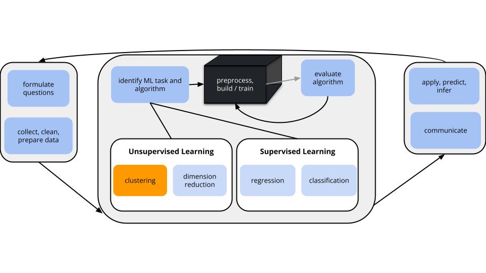
GOALS

Suppose we have a set of feature variables \((x_1,x_2,...,x_p)\) but NO outcome variable \(y\).

Thus instead of our goal being to predict/classify/explain y, we might simply want to…

1. Do a cluster analysis: Examine the structure among the rows, i.e. individual cases or data points, of our data.
2. Utilize this examination as a jumping off point for further analysis.

Techniques: hierarchical clustering & K-means clustering

EXAMPLE

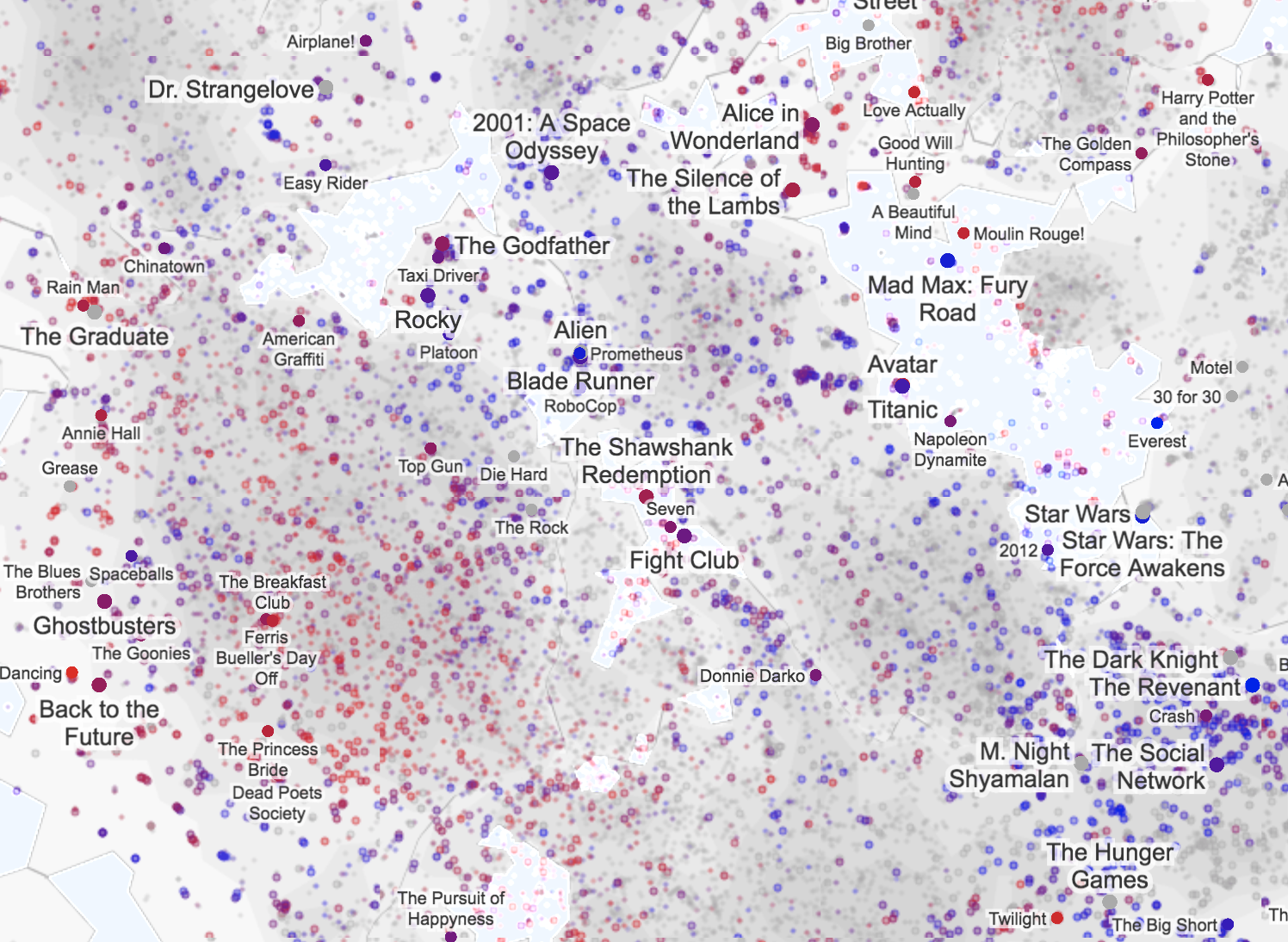
K-means is the clustering technique behind Cartograph.info

Notes: K-means Clustering

Drawbacks of hierarchical clustering

1. can be computationally expensive: we have to calculate the distance between each pair of objects in our sample to start the algorithm

2. greedy algorithm: This algorithm makes the best local decision of which clusters to fuse at each step in the dendrogram. Once clusters are fused they remain fused throughout the dendrogram. However, meaningful clusters may not always be hierarchical or nested.

K-means Clustering

Goal:
Split cases into K non-overlapping, homogeneous clusters or groups of cases noted as \(C_1, C_2,..., C_k\) which minimize the total within_cluster variance:

\[\sum_{k=1}^K W(C_k)\]

where each \(W(\cdot)\) measures the within-cluster variance of each \(C_k\):

\[W(C_k) = \frac{1}{\text{# of cases in $C_k$}} (\text{total Euclidean distance}^2 \text{ btwn all pairs in $C_k$})\]

Specifically, \(W(C_k)\) is the average squared distance between all pairs of cases in cluster \(C_k\).

Algorithm:

0. Pick K
   Appropriate values of K are context dependent and can be deduced from prior knowledge, data, or the results of hierarchical clustering. Try multiple!

1. Initialization
   Randomly select the location of \(K\) centroids. Assign each case to the nearest centroid. This random composition defines the first set of clusters \(C_1\) through \(C_K\).

2. Centroid calculation
   Calculate the centroid, ie. average location of the cases \(x\) in each \(C_i\).

3. Cluster assignment
   Re-assign each case to the \(C_i\) with the nearest centroid.

4. Repeat!
   Iterate between steps 2 and 3 until the clusters stabilize, ie. the cluster centroids do not change much from iteration to iteration.

Small Group Discussion

EXAMPLE 1: revisit the hierarchical algorithm

Recall the hierarchical algorithm.

• Each data point starts as a leaf.
• Compute the Euclidean distance between all pairs of data points with respect to their features x.
• Fuse the 2 closest data points into a single cluster or branch.
• Continue to fuse the 2 closest clusters until all cases are in 1 cluster.

Revisit screenshots from the shiny app to explore the results of this algorithm. Why can the “greediness” of this algorithm sometimes produce strange results?

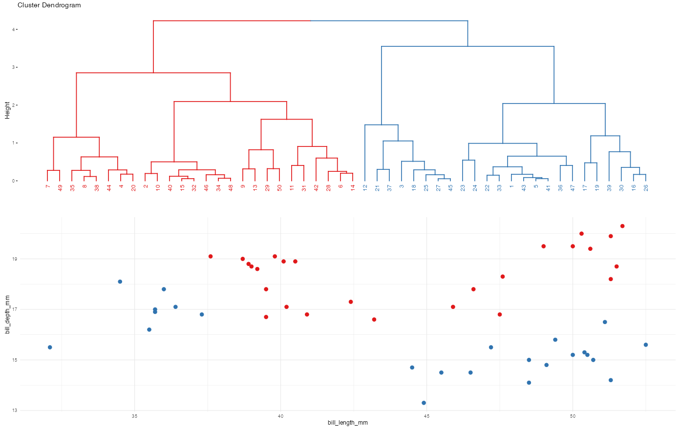
Solution:

Clusters are hierarchical / nested. Once we combine two clusters, we can’t separate them.

EXAMPLE 2: Interact with the K-Means algorithm

Here’s the idea and more details are above:

1. Initialization

   • Pick K, the number of clusters to build.
   • Randomly select the location of K centroids.
   • Assign each data point to the nearest centroid.

2. Centroid calculation
   Calculate the centroid of each cluster.

3. Cluster assignment
   Re-assign each data point to the cluster with the nearest centroid.

4. Repeat! Iterate!
   Iterate between steps 2 and 3 until the clusters stabilize.

Naftali Harris made a really nice interactive app for playing around with this algorithm.

• “How to pick the initial centroids?”: Select “I’ll Choose”
  
• “What kind of data would you like?”: Select “Gaussian Mixture”

You’ll notice 3 natural clusters.

To understand how and if K-means clustering with K = 3 might detect these clusters, play around:

• Initialization & centroid calculation: Click on 3 locations (not on the clusters themselves!) to define starting points for the K = 3 cluster centroids.
• Cluster assignment: Click “GO!” to assign data points to the nearest centroid.
• Centroid calculation: Click “Update Centroids” to recalculate the centroids of the new clusters.
• Cluster assignment: Click “Reassign points” to reassign data points to the nearest centroid.
• Repeat until your clusters stop changing.

Challenge:

Can you identify a set of initial centroids that result in reasonable final clusters? What about a set of initial centroids that don’t result in reasonable final clusters?

Solution:

example of a good K-means outcome
example of a bad K-means outcome

EXAMPLE 3: K-means vs K-means

Let’s do K-means clustering in R using our penguin data:

library(tidyverse)
library(palmerpenguins)
data(penguins)

# For demo only, take a sample of 50 penguins
set.seed(253)
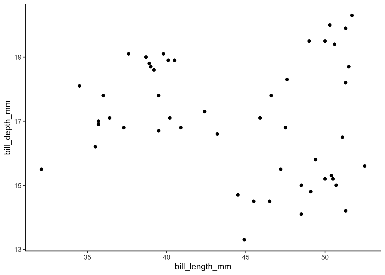
penguins <- sample_n(penguins, 50) %>% 
  select(bill_length_mm, bill_depth_mm)

We’ll cluster these penguins based on their bill lengths and depths:

ggplot(penguins, aes(x = bill_length_mm, y = bill_depth_mm)) + 
  geom_point() 

1. Run the K-means algorithm using K = 3. We didn’t set the seed for hierarchical clustering. Why do we have to set the seed for K-means? Why do we have to scale the data?

   # Run the K-means algorithm
   set.seed(253)
   kmeans_3_round_1 <- kmeans(scale(penguins), centers = 3) 
   
   # Plot the cluster assignments
   penguins %>% 
     mutate(kmeans_cluster = as.factor(kmeans_3_round_1$cluster)) %>%
     ggplot(aes(x = bill_length_mm, y = bill_depth_mm, color = kmeans_cluster)) + 
       geom_point(size = 3) + 
       theme(legend.position = "none") + 
       labs(title = "K-means with K = 3 (round 1)") + 
       theme_minimal()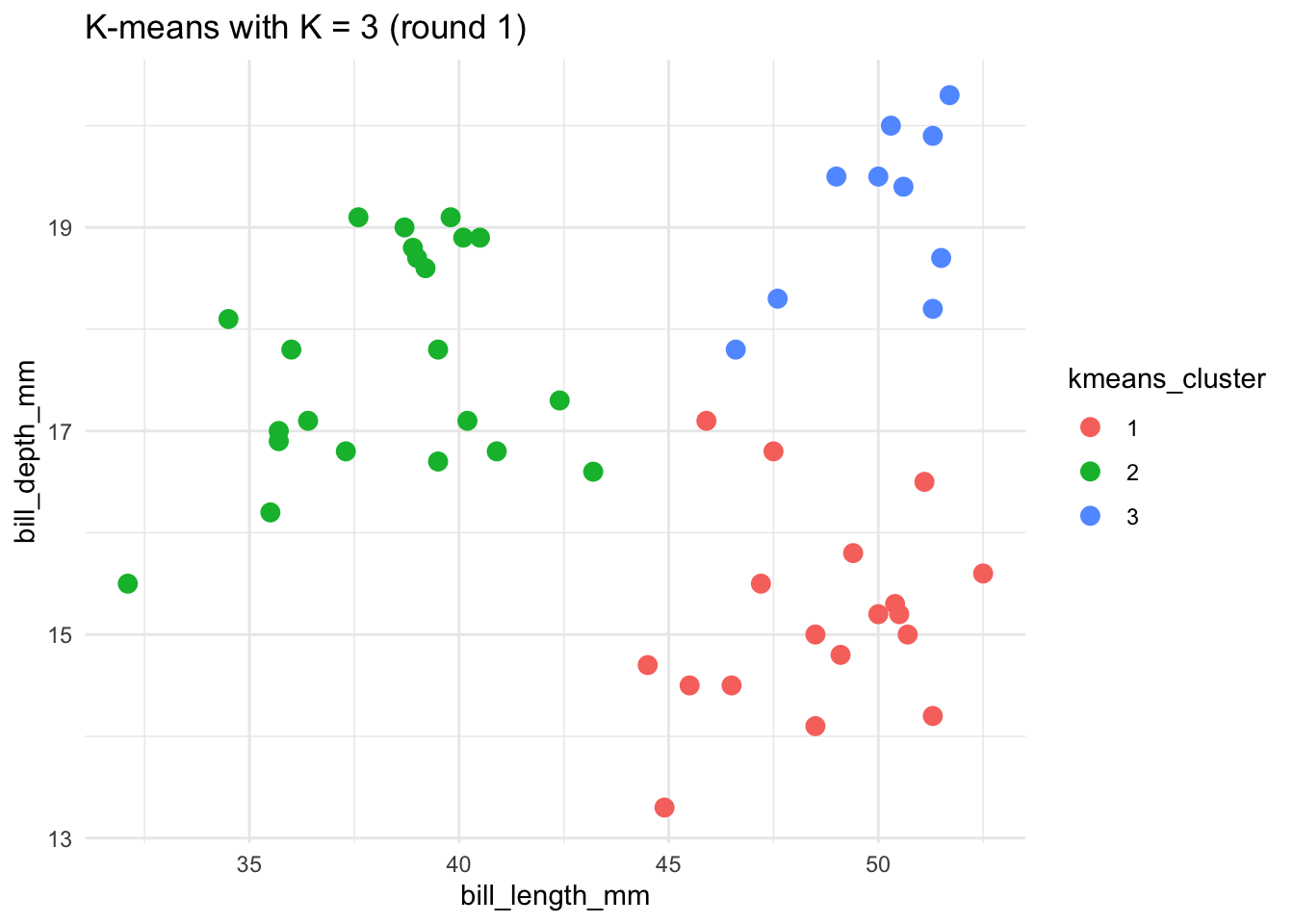

   

2. Let’s repeat the K-means algorithm with K = 3. BUT let’s use a different seed. How did the results change and why is this possible?

   # Run the K-means algorithm using a seed of 8
   set.seed(8)
   kmeans_3_round_2 <- kmeans(scale(penguins), centers = 3) 
   
   # Plot the cluster assignments
   penguins %>% 
     mutate(kmeans_cluster = as.factor(kmeans_3_round_2$cluster)) %>%
     ggplot(aes(x = bill_length_mm, y = bill_depth_mm, color = kmeans_cluster)) + 
       geom_point(size = 3) + 
       theme(legend.position = "none") + 
       labs(title = "K-means with K = 3 (round 2)") + 
       theme_minimal()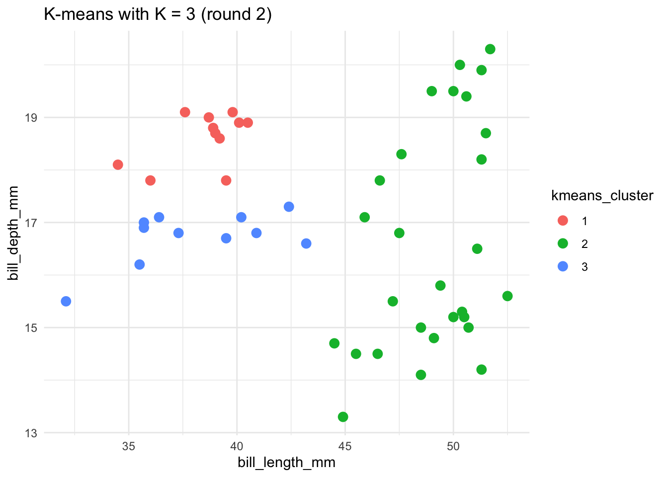

   

3. In practice, why should we try out a variety of seeds?

Solution:

1. The initial centroids are randomly selected. K-means algorithm assigns data point to clusters using distances (we don’t want these assignments to be skewed by the scales of features x).
2. The 2 runs of the K-means started out with different initial centroids and this was enough to produce different results!
3. Make sure our results aren’t overly sensitive to / skewed by the random centroids we happened to start with.

EXAMPLE 4: IMPACT OF K

To implement K-means clustering we must choose an appropriate K! Use the following example to discuss the goldilocks challenge of picking K.

penguins_sub <- penguins %>%
  select(bill_length_mm, bill_depth_mm) %>% 
  na.omit()

# Run K-means
set.seed(253)
k_2  <- kmeans(scale(penguins_sub), centers = 2)
k_20 <- kmeans(scale(penguins_sub), centers = 20)

penguins_sub %>% 
  mutate(cluster_2 = as.factor(k_2$cluster)) %>% 
  ggplot(aes(x = bill_length_mm, y = bill_depth_mm, color = cluster_2)) + 
    geom_point(size = 3) + 
    labs(title = "K = 2")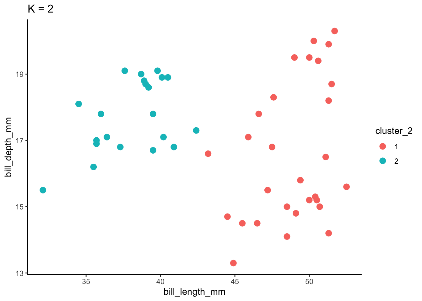

penguins_sub %>% 
  mutate(cluster_20 = as.factor(k_20$cluster)) %>% 
  ggplot(aes(x = bill_length_mm, y = bill_depth_mm, color = cluster_20)) + 
    geom_point(size = 3) + 
    labs(title = "K = 20") + 
    scale_color_manual(values = rainbow(20))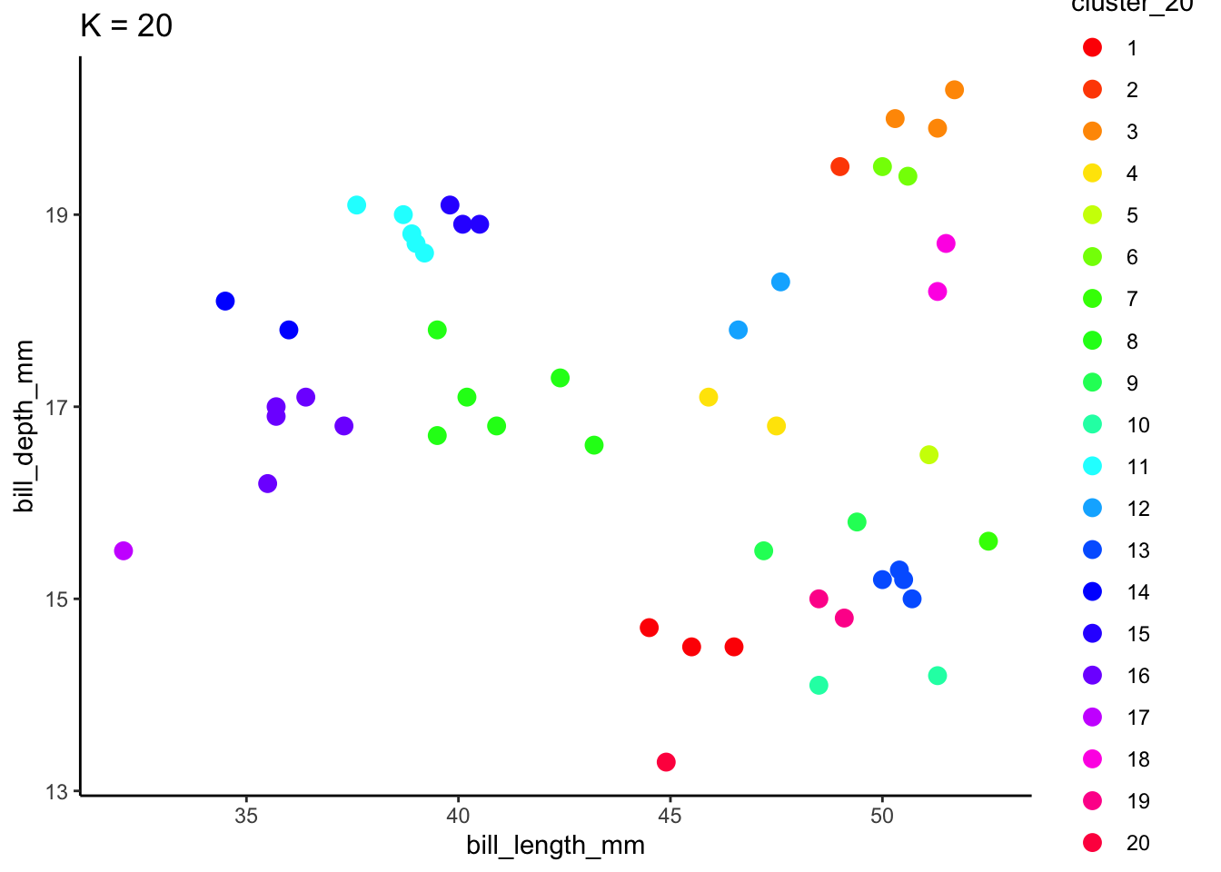

Solution:

When K is too small, we can end up with big and overly general clusters. When K is too big, we can end up with small clusters that are too local / lose the general patterns.

EXAMPLE 5: hierarchical vs K-means

Let’s compare and contrast the results of the hierarchical and K-means algorithms.

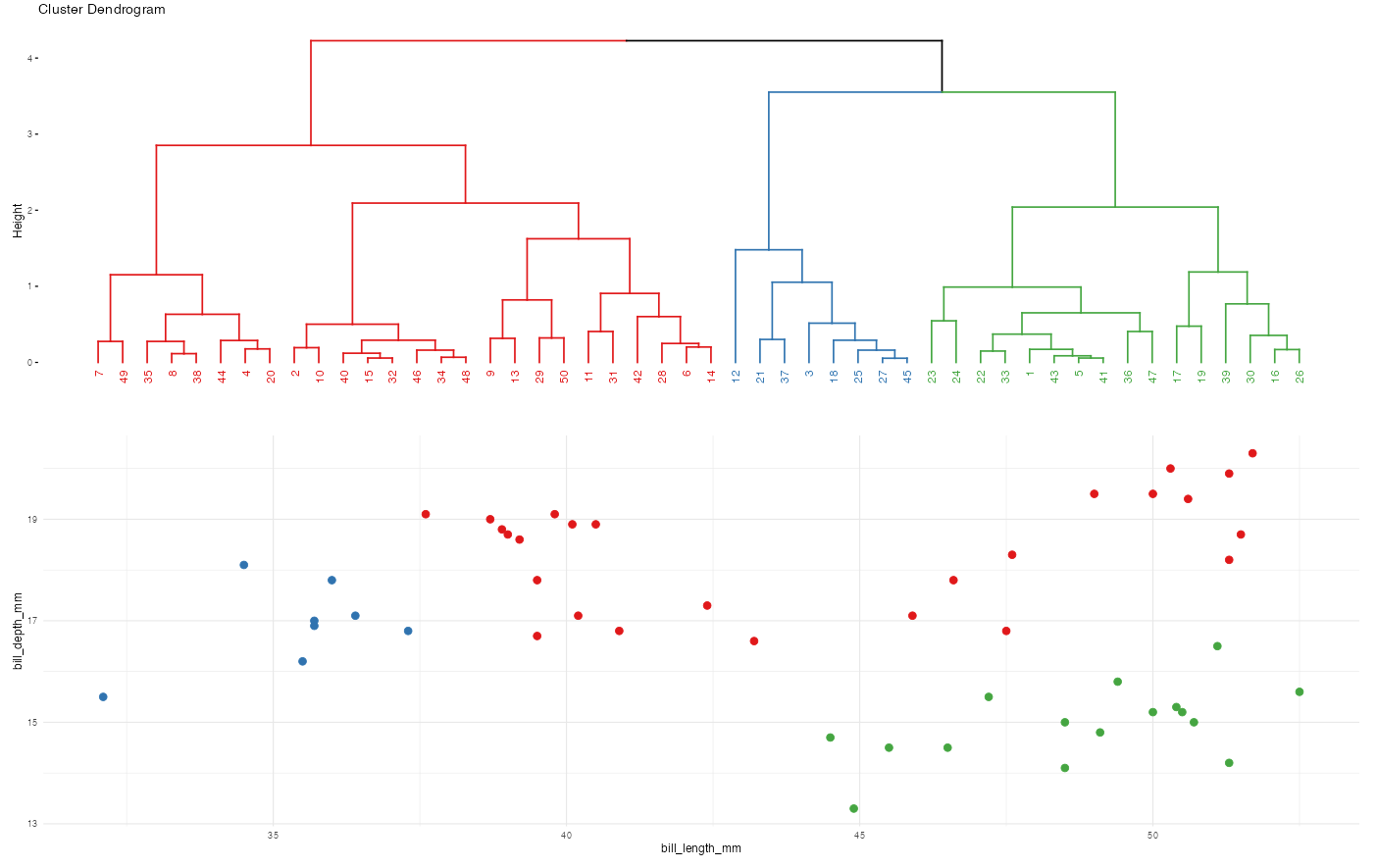
To this end, let’s use both to identify 2 penguin clusters:

# Run hierarchical algorithm
hier_alg <- hclust(dist(scale(penguins)))

# Run K-means
set.seed(253)
kmeans_alg <- kmeans(scale(penguins), centers = 2) 

# Include the clustering assignments
cluster_data <- penguins %>% 
  mutate(
    hier_cluster = as.factor(cutree(hier_alg, 2)),
    kmeans_cluster = as.factor(kmeans_alg$cluster))

1. Do the clusters defined by the two algorithms agree? NOTE: the actual cluster numbers are arbitrary.

   head(cluster_data)

2. Plot the cluster assignments. Which algorithm produces seemingly better clusters?

   ggplot(cluster_data, aes(x = bill_length_mm, y = bill_depth_mm, color = hier_cluster)) + 
     geom_point(size = 3) + 
     labs(title = "hiearchical results") +
     theme(legend.position = "none") + 
     theme_minimal()
   
   ggplot(cluster_data, aes(x = bill_length_mm, y = bill_depth_mm, color = kmeans_cluster)) + 
     geom_point(size = 3) + 
     theme(legend.position = "none") + 
     labs(title = "K-means results") + 
     theme_minimal()

Solution:

1. no
2. K-means is better. The hierarchical clusters are odd – it fused two penguins early on, and could not unfuse them later.

EXAMPLE 6: Pros & Cons

Name 1 pro and 2 drawbacks of the K-means algorithm.

Solution:

• Pro: not greedy
• Cons:
  • We have to pre-specify the number of clusters we’re interested in.
  • We can get different results based on where we put the first centroids.

Bonus

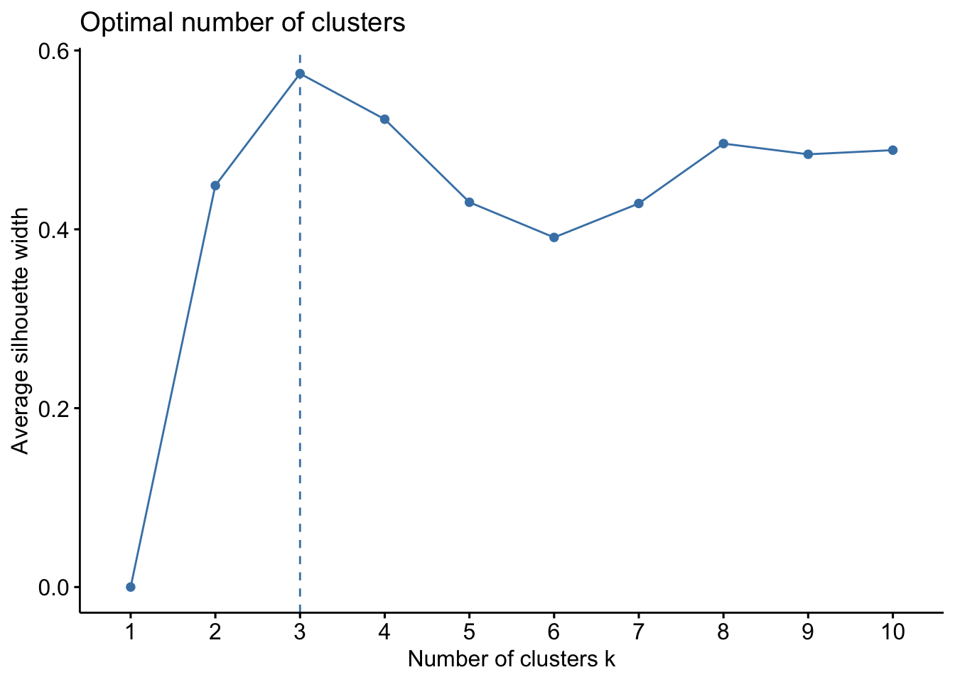
Choosing \(K\) - Average Silhouette

Goal: Choose \(K\) that maximizes the distance between clusters and minimizes distance within clusters

\[a(i) = \frac{1}{|C_I|} \sum_{j\in C_I, i\not=j} ||\mathbf{x}_i - \mathbf{x_j}||^2\] \[ = \text{ avg. within cluster variance or distance from point i}\]

\[b(i) = \min_{J\not=I}\frac{1}{|C_J|} \sum_{j\in C_J} ||\mathbf{x}_i - \mathbf{x_j}||^2\] \[=\text{ min avg. variance / distance from point i to points in another cluster}\]

Silhouette for point \(i\) (\(-1\leq s(i) \leq 1\)):

\[s(i) = \frac{b(i) - a(i)}{\max\{a(i),b(i)\}}\] \[ = \text{relative difference in within and between distance}\] \[ = \text{measure of how tightly clustered a group of points is relative to other groups }\]

Properties of Silhouette

• If \(b(i) >> a(i)\) (distance to other clusters is far relative to distance within cluster), \(s(i) = 1\). This means it is an appropriate cluster.

• If \(b(i) << a(i)\), point \(i\) is more similar to the neighboring cluster than its own (not great), \(s(i) = -1\).

• If \(b(i) = a(i)\), then \(s(i) = 0\). It is more of a flip of a coin of which cluster point i should be in (on the border between 2).

We plot the average silhouette, \(\frac{1}{n}\sum_{i=1}^n s(i)\), and choose \(K\) that maximizes the average silhouette.

library(factoextra)
fviz_nbclust(scale(penguins), kmeans, method='silhouette')

Exercises

NOTE: These exercises are on Homework 7.

4. Choosing K
   You’ve already run the hierarchical clustering algorithm for the candy data. Let’s try K-means! The first step is to pick K. So how do we choose?
   1. Run and store a K-means algorithm using K = 2. Set the seed to 253.
      
   2. One strategy for evaluating our choice of K is to calculate the total squared distance of each candy from its assigned centroid: the total within- cluster sum of squares. Report this value for your algorithm from part a.
      
   3. Next, calculate the total sum of squared distances for each K in 1, 2, …, n where you pick a reasonable n. Don’t print them, rather, construct a plot of these distances by K.
      
   4. Based on this plot, which values of K seem reasonable? Explain.

5. A final K-means model
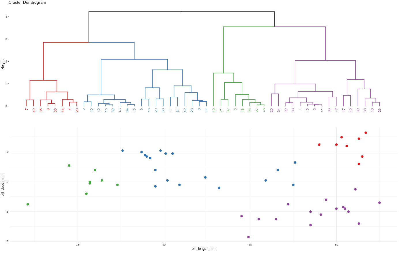
   1. Another strategy for identifying a reasonable number of clusters K for K-means is to do hierarchical clustering, and use the dendrogram to suggest K. Given our earlier choice of using 4 clusters from the dendrogram, run the K-means algorithm using K = 4. Set the seed to 253.
      
   2. To get a sense for what makes the candies in each cluster “similar”, calculate the mean of each feature within each cluster.

6. Final clustering reflection
   1. Do your K-means and hierarchical approaches lead to similar conclusions? (What’s the same? What’s different?)
      
   2. Though K-means is more computationally efficient and less greedy, what’s one pro of hierarchical clustering?
      
   3. Bringing it all together across your various hierarchical and K-means clustering outcomes, offer a set of final conclusions. Specifically, write out a label for each final cluster that communicates its unique properties (eg: “big penguins”, “really big penguins”, and “small penguins with long bills”). NOTE: Focus on the K-means results.

R code

The tidymodels package is built for models of some outcome variable y. We can’t use it for clustering.

Instead, we’ll use a variety of new packages that use specialized, but short, syntax.

Suppose we have a set of sample_data with multiple feature columns x, and (possibly) a column named id which labels each data point.

# Install packages
library(tidyverse)
library(cluster)      # to build the hierarchichal clustering algorithm
library(factoextra)   # to draw the dendrograms

PROCESS THE DATA

If there’s a column that’s an identifying variable or label, not a feature of the data points, convert it to a row name.

sample_data <- sample_data %>% 
  column_to_rownames("id")

K-means can’t handle NA values! There are a couple options.

# Omit missing cases (this can be bad if there are a lot of missing points!)
sample_data <- na.omit(sample_data)

# Impute the missing cases
library(VIM)
sample_data <- sample_data %>%
  VIM::kNN(imp_var = FALSE)

IF you have at least 1 categorical / factor feature, you’ll need to pre-process the data even further. You should NOT do this if you have quantitative and/or logical features.

# Turn categorical features into dummy variables
sample_data <- data.frame(model.matrix(~ . - 1, sample_data))

RUN THE K-MEANS ALGORITHM FOR SPECIFIC K

# K-means clustering
set.seed(___)
kmeans_model <- kmeans(scale(sample_data), centers = ___)


# Get the "the total within- cluster sum of squares"
# This is the total squared distance of each case from its assigned centroid
kmeans_model$tot.withinss

TUNING K-MEANS: TRY A BUNCH OF K

Calculate the total within-cluster sum of squares (SS) for each possible number of clusters K from 1 to n.

# You pick n!!!
tibble(K = 1:n) %>%
  mutate(SS = map(K, ~ kmeans(scale(sample_data), centers = .x)$tot.withinss)) %>% 
  unnest(cols = c(SS))

DEFINING CLUSTER ASSIGNMENTS

# Assign each sample case to a cluster
# We typically want to store this in a new dataset so that the cluster assignments aren't 
# accidentally used as features in a later analysis!
cluster_data <- sample_data %>% 
  mutate(kmeans_cluster_k = kmeans_model$cluster)