Topic 6 LASSO: Shrinkage/Regularization

Learning Goals

Explain how ordinary and penalized least squares are similar and different with regard to (1) the form of the objective function and (2) the goal of variable selection
Explain why variable scaling is important for the performance of shrinkage methods
Explain how the lambda tuning parameter affects model performance and how this is related to overfitting
Describe how output from LASSO models can give a measure of variable importance

Notes: LASSO

CONTEXT

world = supervised learning
We want to model some output variable \(y\) using a set of potential predictors (\(x_1, x_2, ..., x_p\)).
task = regression
\(y\) is quantitative
model = linear regression
We’ll assume that the relationship between \(y\) and (\(x_1, x_2, ..., x_p\)) can be represented by

\[y = \beta_0 + \beta_1 x_1 + \beta_2 x_2 + ... + \beta_p x_p + \varepsilon\]
estimation algorithm = LASSO

LASSO: least absolute shrinkage and selection operator

Goal

Use the LASSO algorithm to help us regularize and select the “best” predictors \(x\) to use in a predictive linear regression model of \(y\):

\[y = \hat{\beta}_0 + \hat{\beta}_1 x_1 + \cdots + \hat{\beta}_p x_p + \varepsilon\]

Idea

Penalize a predictor for adding complexity to the model (by penalizing its coefficient). Then track whether the predictor’s contribution to the model (lowering RSS) is enough to offset this penalty.

Criterion

Identify the model coefficients \(\hat{\beta}_1, \hat{\beta}_2, ... \hat{\beta}_p\) that minimize the penalized residual sum of squares:

\[RSS + \lambda \sum_{j=1}^p \vert \hat{\beta}_j\vert = \sum_{i=1}^n (y_i - \hat{y}_i)^2 + \lambda \sum_{j=1}^p \vert \hat{\beta}_j\vert\]

where

residual sum of squares (RSS) measures the overall model prediction error
the penalty term measures the overall size of the model coefficients
\(\lambda \ge 0\) (“lambda”) is a tuning parameter

Small Group Discussion

EXAMPLE 1: LASSO vs other algorithms for building linear regression models

LASSO vs least squares
- What’s one advantage of LASSO vs least squares?
- Which algorithm(s) require us (or R) to scale the predictors?
What is one advantage of LASSO vs backward stepwise selection?

Solution

LASSO helps with model selection, i.e. kicks some predictors out of the model, and preventing overfitting.
LASSO isn’t greedy and doesn’t overestimate the significance of the predictors it retains (its variable selection isn’t based on p-values).

EXAMPLE 2: LASSO tuning

We have to pick a \(\lambda\) penalty tuning parameter for our LASSO model. What’s the impact of \(\lambda\)?

When \(\lambda\) is 0, …
As \(\lambda\) increases, the predictor coefficients ….
Goldilocks problem: If \(\lambda\) is too big, …. If \(\lambda\) is too small, …
To decide between a LASSO that uses \(\lambda = 0.01\) vs \(\lambda = 0.1\) (for example), we can ….

Solution

LASSO is equivalent to least squares.
shrink toward or to 0.
too big: all predictors are kicked out of the model. too small: too few predictors are kicked out, hence the model is complicated and maybe overfit.
compare CV MAE of the LASSOs with these \(\lambda\)

COMMENT: Picking \(\lambda\)

We cannot know the “best” value for \(\lambda\) in advance. This varies from analysis to analysis.

We must try a reasonable range of possible values for \(\lambda\). This also varies from analysis to analysis.

In general, we have to use trial-and-error to identify a range that is…

wide enough that it doesn’t miss the best values for \(\lambda\)
narrow enough that it focuses on reasonable values for \(\lambda\)

In-Class Activity - Exercises

We’ll use the LASSO algorithm to help us build a good predictive model of height using the collection of 12 possible predictors in the humans dataset:

# Load packages
library(tidyverse)
library(tidymodels)

# Resolves package conflicts by preferring tidymodels functions
tidymodels_prefer()

# Load data
humans <- read.csv("https://bcheggeseth.github.io/253_spring_2024/data/bodyfat2.csv")

Let’s implement the LASSO. We’ll pause to examine the code. The R code section and R code tutorial provide more detail, so no need to take notes here.

# STEP 1: LASSO algorithm / model specification
lasso_spec <- linear_reg() %>%             
  set_mode("regression") %>% 
  set_engine("glmnet") %>%                 
  set_args(mixture = 1, penalty = tune())

# STEP 2: variable recipe
# NOTE: We'll discuss step_dummy() next class.
variable_recipe <- recipe(height ~ ., data = humans) %>% 
  step_dummy(all_nominal_predictors())

# STEP 3: workflow specification (model + recipe)
lasso_workflow <- workflow() %>% 
  add_recipe(variable_recipe) %>% 
  add_model(lasso_spec)

# STEP 4: Estimate 50 LASSO models using different lambda values 
# on a "grid" or range from 10^(-5) to 10^(-0.1).
# Calculate the CV MAE for each of the 50 models.
# NOTE: I usually start with a range from 10^(-5) to 10^1 and tweak through trial-and-error.
set.seed(253)
lasso_models <- lasso_workflow %>% 
  tune_grid(
    grid = grid_regular(penalty(range = c(-5, -0.1)), levels = 50),  
    resamples = vfold_cv(humans, v = 10),   
    metrics = metric_set(mae)
  )

Examining the impact of \(\lambda\)

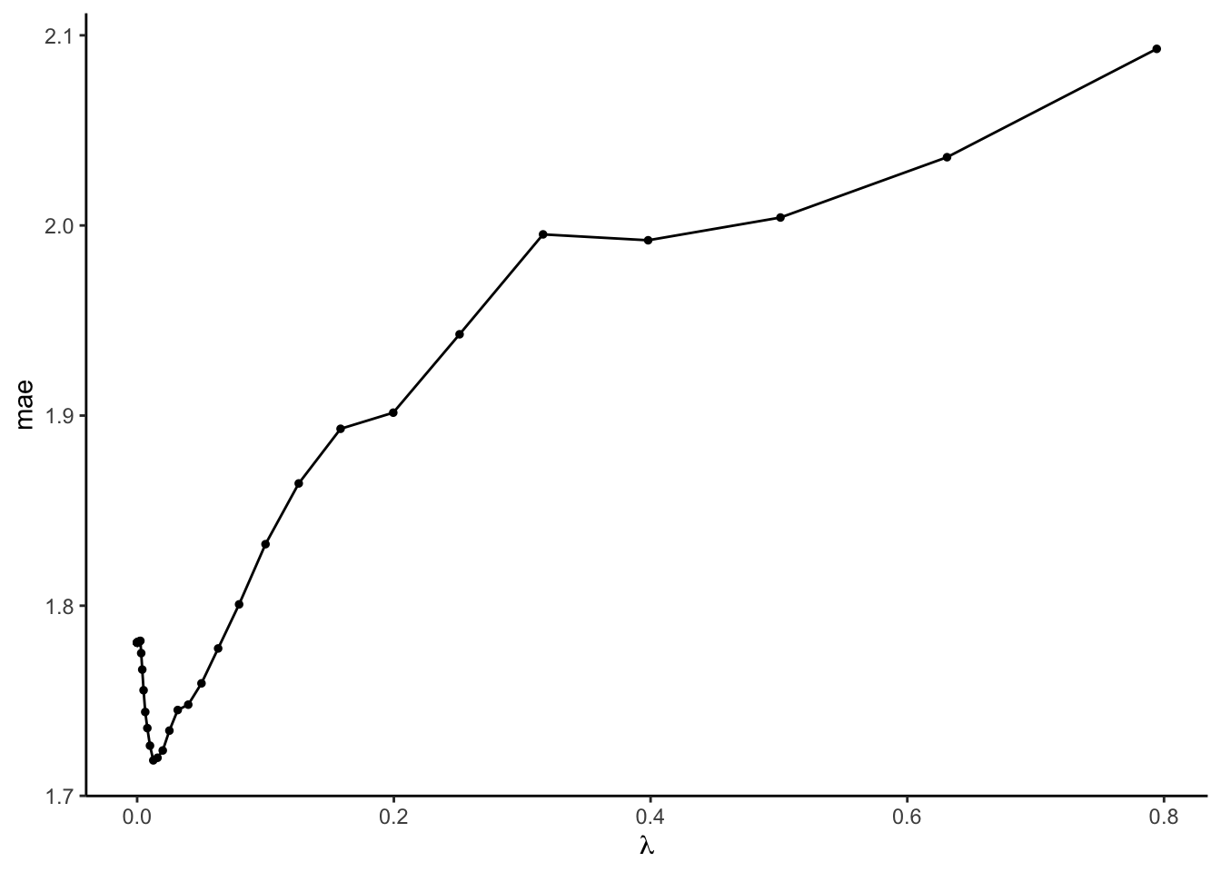
Let’s compare the CV MAEs (y-axis) for our 50 LASSO models which used 50 different \(\lambda\) values (x-axis):

autoplot(lasso_models) + 
  scale_x_continuous() + 
  xlab(expression(lambda))

We told R to use a range of \(\lambda\) from -5 to -0.1 on the log10 scale. Calculate this range on the non-log scale and confirm that it matches the x-axis.

10^(-5)
10^(-0.1)

Explain why this plot displays the “goldilocks” problem of tuning \(\lambda\).

Solution

autoplot(lasso_models) + 
  scale_x_continuous() + 
  xlab(expression(lambda))

Yep it matches.

10^(-5)

## [1] 1e-05

10^(-0.1)

## [1] 0.7943282

CV MAE is large when \(\lambda\) is either too small or too big.

Picking a \(\lambda\) value

In the plot above, roughly which value of the \(\lambda\) penalty parameter produces the smallest CV MAE? Check your approximation:

best_penalty <- lasso_models %>% 
  select_best(metric = "mae")

best_penalty

Suppose we prefer a parsimonious model. The plot below adds error bars to the CV MAE estimates of prediction error (+/- one standard error). Any model with a CV MAE that falls within another model’s error bars is not significantly better or worse at prediction:

# With error bars
autoplot(lasso_models) + 
  scale_x_continuous() + 
  xlab(expression(lambda)) + 
  geom_errorbar(data = collect_metrics(lasso_models),
  aes(x = penalty, ymin = mean - std_err, ymax = mean + std_err), alpha = 0.5)

Use this to approximate the largest \(\lambda\), thus the most simple LASSO model, that produces a CV MAE that’s within 1 standard error of the best model (thus is not significantly worse). Check your approximation:

parsimonious_penalty <- lasso_models %>% 
  select_by_one_std_err(metric = "mae", desc(penalty))
parsimonious_penalty

Moving forward, we’ll use the parsimonious LASSO model. Simply report the tuning parameter \(\lambda\) here. Just as a radio show needs to tell its audience where to tune the radio dial, it’s important to explicitly report \(\lambda\) so that we and others can reproduce the model!

Solution

\(\lambda\) close to 0

best_penalty <- lasso_models %>% 
select_best(metric = "mae")
best_penalty

## # A tibble: 1 × 2
##   penalty .config              
##     <dbl> <chr>                
## 1  0.0126 Preprocessor1_Model32

\(\lambda\) around 0.2

# With error bars
autoplot(lasso_models) + 
  scale_x_continuous() + 
  xlab(expression(lambda)) + 
  geom_errorbar(data = collect_metrics(lasso_models),
                aes(x = penalty, ymin = mean - std_err, ymax = mean + std_err), alpha = 0.5)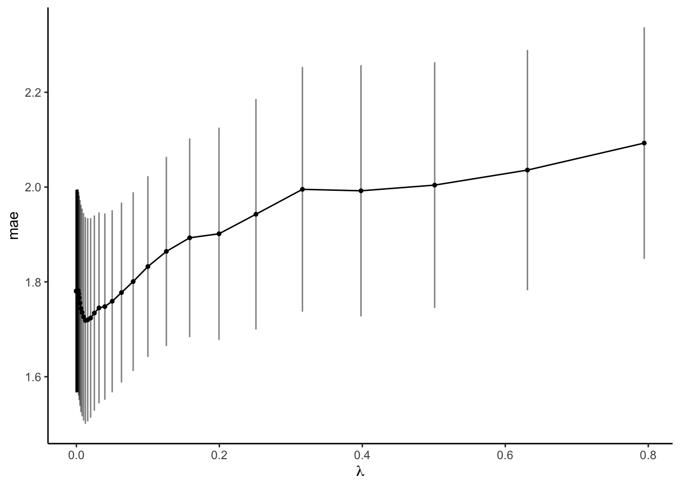

parsimonious_penalty <- lasso_models %>% 
  select_by_one_std_err(metric = "mae", desc(penalty))
parsimonious_penalty

## # A tibble: 1 × 9
##   penalty .metric .estimator  mean     n std_err .config        .best .bound
##     <dbl> <chr>   <chr>      <dbl> <int>   <dbl> <chr>          <dbl>  <dbl>
## 1   0.200 mae     standard    1.90    10   0.224 Preprocessor1…  1.72   1.94

PAUSE: Picking a range to try for \(\lambda\)

The range of values we tried for \(\lambda\) had the following nice properties. If it didn’t, we should adjust our range (make it narrower or wider).

Our range was wide enough.
We observed the goldilocks effect. Further, the “best” and “parsimonious” \(\lambda\) values were not at the edges of the range, suggesting there aren’t better \(\lambda\) values outside our range.

Our range was narrow enough.
We didn’t observe any loooooong flat lines in CV MAE, thus we narrowed in on the \(\lambda\) values where the “action is happening”, i.e. where changing \(\lambda\) impacts the model.

Finalizing our LASSO model

Let’s finalize our parsimonious LASSO model:

final_lasso <- lasso_workflow %>% 
  finalize_workflow(parameters = parsimonious_penalty) %>% 
  fit(data = humans)
    
final_lasso %>% 
  tidy()

How many and which predictors were kept in this model?
How do these compare to the 5-predictor model we identify using the backward stepwise selection algorithm with this subset of data: weight, abdomen, thigh, neck, chest
Through shrinkage, the LASSO coefficients lose some contextual meaning, so we typically shouldn’t interpret them. Why don’t we care?! THINK: What is the goal of LASSO modeling?
The LASSO tidy() summary doesn’t report p-values for testing the “significance” of our predictors. Why don’t we care? (Name two reasons.)

Solution

final_lasso <- lasso_workflow %>% 
  finalize_workflow(parameters = parsimonious_penalty) %>% 
  fit(data = humans)

final_lasso %>% 
  tidy() %>% 
  filter(estimate != 0)

## # A tibble: 6 × 3
##   term        estimate penalty
##   <chr>          <dbl>   <dbl>
## 1 (Intercept)  63.8      0.200
## 2 weight        0.0696   0.200
## 3 abdomen      -0.126    0.200
## 4 thigh        -0.0199   0.200
## 5 knee          0.156    0.200
## 6 ankle         0.0474   0.200

5: weight, abdomen, thigh, knee, ankle
3 of the predictors are the same. LASSO includes knee (which is the most highly correlated with height in this dataset)
We’re using this model to give good predictions, not to explore / make inferences about relationships.
The remaining predictors are those that have significant predictive power in this linear regression model (thus we get conclusions like a hypothesis test without doing a test). Our goal is to build a good predictive model, not to do inference.

LASSO vs LASSO

Our parsimonious LASSO selected only 5 of the 12 possible predictors. Out of curiosity, how many predictors would have remained if we had used the best_penalty value for \(\lambda\)?

lasso_workflow %>% 
  finalize_workflow(parameters = ___) %>% 
  fit(data = humans) %>% 
  tidy()

Based on this example, do you think LASSO is a greedy algorithm? Are you “stuck” with your past locally optimal choices? Compare the predictors in this larger model with those in the smaller, parsimonious model.

Solution

This would have 11 predictors.

lasso_workflow %>% 
  finalize_workflow(parameters = best_penalty) %>% 
  fit(data = humans) %>% 
  tidy() %>% 
  filter(estimate != 0)

## # A tibble: 12 × 3
##    term        estimate penalty
##    <chr>          <dbl>   <dbl>
##  1 (Intercept) 104.      0.0126
##  2 age          -0.0208  0.0126
##  3 weight        0.243   0.0126
##  4 neck         -0.595   0.0126
##  5 chest        -0.102   0.0126
##  6 abdomen      -0.200   0.0126
##  7 hip          -0.0491  0.0126
##  8 thigh        -0.307   0.0126
##  9 knee          0.180   0.0126
## 10 biceps       -0.145   0.0126
## 11 forearm      -0.0640  0.0126
## 12 wrist        -0.0864  0.0126

ankle is not in this larger model but it is in the more parsimonious model. Therefore, the algorithm can’t be greedy. If it were greedy, then ankle would get removed for all smaller models.

LASSO vs least squares

Let’s compare our final_lasso model to the least squares model using all predictors:

# Build the LS model
lm_spec <- linear_reg() %>% 
  set_mode("regression") %>% 
  set_engine("lm")

ls_workflow <- workflow() %>%
  add_model(lm_spec) %>%
  add_recipe(variable_recipe)

ls_model <- ls_workflow %>% 
  fit(data = humans) 

ls_model %>% 
  tidy()

set.seed(253)
ls_workflow %>% 
  fit_resamples(
    resamples = vfold_cv(humans,v = 10),
    metrics = metric_set(mae)
  ) %>% collect_metrics()

Our final_lasso has 5 predictors and a CV MAE of 1.90 (calculated above). The ls_model has 12 predictors and a CV MAE of 1.80. Comment.
Use both final_lasso and ls_model to predict the height of the new patient below. How do these compare? Does this add to or calm any fears you might have had about shrinking coefficients?!

new_patient <- data.frame(age = 50, weight = 200, neck = 40, chest = 115, abdomen = 105, hip = 100, thigh = 60, knee = 38, ankle = 23, biceps = 32, forearm = 29, wrist = 19)

# LS prediction
___ %>% 
predict(new_data = ___)

# LASSO prediction
___ %>% 
predict(new_data = ___)

Which final model would you choose, the LASSO or least squares?

Solution

# Build the LS model
lm_spec <- linear_reg() %>% 
  set_mode("regression") %>% 
  set_engine("lm")

ls_workflow <- workflow() %>%
  add_model(lm_spec) %>%
  add_recipe(variable_recipe)

ls_model <- ls_workflow %>% 
  fit(data = humans) 

ls_model %>% 
  tidy()

## # A tibble: 13 × 5
##    term        estimate std.error statistic     p.value
##    <chr>          <dbl>     <dbl>     <dbl>       <dbl>
##  1 (Intercept) 110.       16.9       6.51   0.000000561
##  2 age          -0.0234    0.0367   -0.637  0.529      
##  3 weight        0.266     0.0573    4.64   0.0000810  
##  4 neck         -0.671     0.335    -2.00   0.0556     
##  5 chest        -0.119     0.131    -0.908  0.372      
##  6 abdomen      -0.196     0.113    -1.73   0.0946     
##  7 hip          -0.0978    0.189    -0.518  0.609      
##  8 thigh        -0.313     0.163    -1.92   0.0661     
##  9 knee          0.199     0.272     0.733  0.470      
## 10 ankle        -0.0262    0.449    -0.0583 0.954      
## 11 biceps       -0.168     0.200    -0.837  0.410      
## 12 forearm      -0.0770    0.144    -0.536  0.596      
## 13 wrist        -0.0962    0.647    -0.149  0.883

set.seed(253)
ls_workflow %>% 
  fit_resamples(
    resamples = vfold_cv(humans,v = 10),
    metrics = metric_set(mae)
  ) %>% collect_metrics()

## # A tibble: 1 × 6
##   .metric .estimator  mean     n std_err .config             
##   <chr>   <chr>      <dbl> <int>   <dbl> <chr>               
## 1 mae     standard    1.81    10   0.212 Preprocessor1_Model1

LASSO model is much simpler, and has only slightly worse predictions (on the scale of inches).
They’re very similar! Shrinking coefficients doesn’t mean our predictions are odd.

new_patient <- data.frame(age = 50, weight = 200, neck = 40, chest = 115, abdomen = 105, hip = 100, thigh = 60, knee = 38, ankle = 23, biceps = 32, forearm = 29, wrist = 19) 

# LS prediction
ls_model %>% 
  predict(new_data = new_patient)

## # A tibble: 1 × 1
##   .pred
##   <dbl>
## 1  70.1

# LASSO prediction
final_lasso %>% 
  predict(new_data = new_patient)

## # A tibble: 1 × 1
##   .pred
##   <dbl>
## 1  70.3

LASSO

Visualizing LASSO shrinkage

Finally, let’s zoom back out and compare the coefficients for all 50 LASSO models:

# Get output for each LASSO model
all_lassos <- final_lasso %>% 
  extract_fit_parsnip() %>%
  pluck("fit")
    
# Plot coefficient paths as a function of lambda
plot(all_lassos, xvar = "lambda", label = TRUE, col = rainbow(20))
    
# Codebook for which variables the numbers correspond to
rownames(all_lassos$beta)

There’s a lot of information in this plot!

lines = each line represents a different predictor. The small number to the left of each line indicates the predictor by its order in the rownames() list. Click “Zoom” to zoom in.
x-axis = our range of \(\lambda\) values, on the log scale
y-axis = coefficient values at the corresponding \(\lambda\)
numbers above the plot = how many predictors remain in the model with the corresponding \(\lambda\)

We’ll process this information in the next 2 exercises.

#Here is code to recreate that plot
lasso_coefs <- all_lassos$beta  %>% 
  as.matrix() %>%  
  t() %>% 
  as.data.frame() %>% 
  mutate(lambda = all_lassos$lambda ) %>%
  pivot_longer(cols = -lambda, 
               names_to = "term", 
               values_to = "coef")

lasso_coefs %>% filter(coef != 0, lambda > 1)

lasso_coefs %>%
  ggplot(aes(x = lambda, y = coef, color = term)) +
  geom_line() +
  geom_text(data = lasso_coefs %>% filter(lambda == min(lambda)), aes(x = 0.001, label = term), size = 2) + 
  scale_x_log10(limits = c(-2, 2)) +
  guides(color = FALSE)

plot: examining specific predictors

Answer the following questions for predictor 7.

Which predictor is this?
Approximate the coefficient in the LASSO with \(log(\lambda) \approx -5\).
At what \(log(\lambda)\) does the coefficient start to significantly shrink?
At what \(log(\lambda)\) does the predictor get dropped from the model?

Solution

# Get output for each LASSO model
all_lassos <- final_lasso %>% 
  extract_fit_parsnip() %>%
  pluck("fit")

# Plot coefficient paths as a function of lambda
plot(all_lassos, xvar = "lambda", label = TRUE, col = rainbow(20))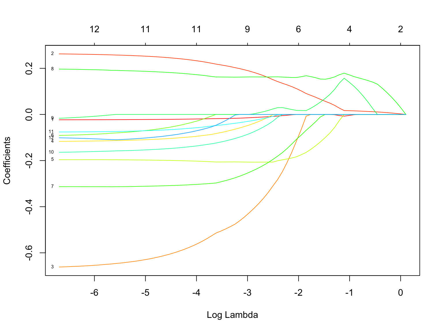

# Codebook for which variables the numbers correspond to
rownames(all_lassos$beta)

##  [1] "age"     "weight"  "neck"    "chest"   "abdomen" "hip"     "thigh"  
##  [8] "knee"    "ankle"   "biceps"  "forearm" "wrist"

thigh
very roughly -0.32
roughly -3.5
roughly -1.8

plot: big picture

How does this plot reflect the LASSO shrinkage phenomenon?
What is one of the most “important” or “persistent” predictors?
What is one of the least persistent predictors?
Our parsimonious LASSO model had 5 predictors. How many predictors would remain if we had minimized the CV MAE using \(\lambda \approx 0.0126\) (\(log(\lambda) = -4.4\))?

Solution

coefficients are shrinking toward or to 0 as \(\lambda\) increases
weight (variable 2), knee (variable 8)
lots of options here. look for the lines that drop to 0 sooner.
11

REVIEW: Model evaluation

Let’s finalize our LASSO analysis. Just as in least squares, it’s important to evaluate a LASSO model before applying it. We’ve already examined whether our LASSO model produces accurate predictions. Use a residual plot to determine if this model is wrong. NOTE: augment() gives predictions, but not residuals :/. You’ll need to calculate them.

# Note what augment() gives us
final_lasso %>% 
  augment(new_data = humans) %>% 
  names()

# Now calculate and plot the residuals
final_lasso %>% 
  augment(new_data = humans) %>% 
  mutate(.resid = ___) %>% 
  ggplot(aes(x = ___, y = ___)) + 
  geom_point() + 
  geom_hline(yintercept = 0)

Solution

final_lasso %>% 
  augment(new_data = humans) %>% 
  names()

##  [1] "age"     "weight"  "neck"    "chest"   "abdomen" "hip"     "thigh"  
##  [8] "knee"    "ankle"   "biceps"  "forearm" "wrist"   "height"  ".pred"

# Now calculate and plot the residuals
final_lasso %>% 
  augment(new_data = humans) %>% 
  mutate(.resid = height - .pred) %>% 
  ggplot(aes(x = .pred, y = .resid)) + 
  geom_point() + 
  geom_hline(yintercept = 0) + 
  geom_smooth(se = FALSE)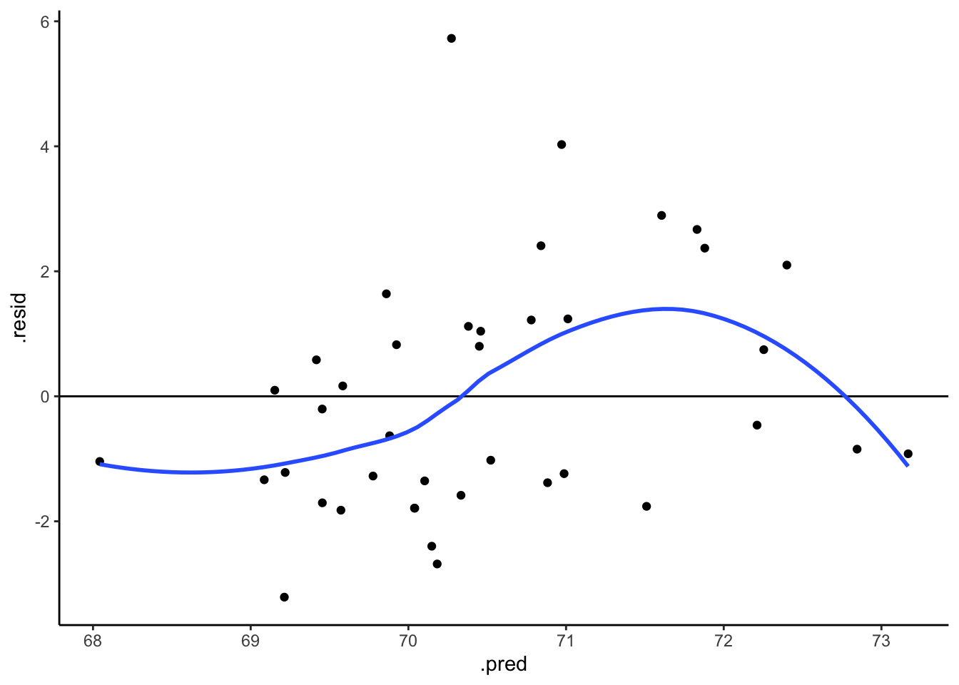

OPTIONAL: Practice on another dataset.

The Hitters data in the ISLR package contains the salaries and performance measures for 322 Major League Baseball players. Use LASSO to determine the “best” predictive model of player Salary.

# Load the data
library(ISLR)
data(Hitters)
Hitters <- Hitters %>% 
  filter(!is.na(Salary))

# IN THE CONSOLE (not in the Rmd): Examine codebook
#?Hitters

Reflection
This is the end of the (short!) Unit 2 on “Regression: Model Selection”! Let’s reflect on the technical content of this unit:
- What was the main motivation / goal behind this unit?
- For each of the following algorithms, describe the steps, pros, cons, and comparisons to least squares:
  - best subset selection
  - backward stepwise selection
  - LASSO
- In your own words, define the following: parsimonious models, greedy algorithms, goldilocks problem.
- Review the new tidymodels syntax from this unit. Identify key themes and patterns.

Deeper learning (very optional)

If you’re curious, consider how the LASSO connects to some other algorithms we won’t cover in STAT 253.

RIDGE REGRESSION

LASSO isn’t the only shrinkage & regularization algorithm. An alternative is ridge regression. This algorithm also seeks to build a (predictive) linear regression model of \(y\):

\[y = \hat{\beta}_0 + \hat{\beta}_1 x_1 + \cdots + \hat{\beta}_p x_p + \varepsilon\]

It also does so by selecting coefficients which minimize a penalized residual sum of squares. HOWEVER, the ridge regression penalty is based upon the sum of squared coefficients instead of the sum of absolute coefficients:

\[RSS + \lambda \sum_{j=1}^p \hat{\beta}_j^2\]

This penalty regularizes / shrinks the coefficients. BUT, unlike the LASSO, ridge regression does NOT shrink coefficients to 0, thus cannot be used for variable selection. (Check out the ISLR text for a more rigorous, geometric explanation for why LASSO often shrinks coefficients to 0.)

ELASTIC NET

The elastic net is yet another shrinkage & regularization algorithm. It combines the penalties used in LASSO and ridge regression. This algorithm seeks to build a (predictive) linear regression model of \(y\):

\[y = \hat{\beta}_0 + \hat{\beta}_1 x_1 + \cdots + \hat{\beta}_p x_p + \varepsilon\]

by selecting coefficients which minimize the following penalized residual sum of squares:

\[RSS + \lambda_1 \sum_{j=1}^p \vert \hat{\beta}_j \vert + \lambda_2 \sum_{j=1}^p \hat{\beta}_j^2\]

NOTE:

Elastic net depends upon two tuning parameters, \(\lambda_1\) and \(\lambda_2\), thus is more complicated than the LASSO.
In cases when we have a group of correlated predictors, LASSO tends to select only one of these predictors. The elastic net does not.

BAYESIAN CONNECTIONS

IF you have taken or will take Bayesian statistics (STAT 454), we can also write the LASSO as a Bayesian model. Specifically, LASSO estimates are equivalent to the posterior mode estimates of \(\beta_j\).

\[\begin{split} Y_i | \beta_0,...\beta_k & \sim N(\beta_0 + \beta_1X_1 + \cdots + \beta_p X_p, \sigma^2) \\ \beta_j & \sim \text{ Laplace (double-exponential)}(0, f(\lambda)) \\ \sigma^2 & \sim \text{ some prior} \\ \end{split}\]

Notes - R code

Suppose we want to build a model of response variable y using all possible predictors in our sample_data.

# Load packages
library(tidymodels)

Build the model for a range of tuning parameters

# STEP 1: LASSO model specification
lasso_spec <- linear_reg() %>% 
  set_mode("regression") %>% 
  set_engine("glmnet") %>% 
  set_args(mixture = 1, penalty = tune())

STEP 1 notes:

We use the glmnet, not lm, engine to build the LASSO.
The glmnet engine requires us to specify some arguments (set_args):
- mixture = 1 indicates LASSO. Changing this would run a different regularization algorithm.
- penalty = tune() indicates that we don’t (yet) know an appropriate \(\lambda\) penalty term. We need to tune it.

# STEP 2: variable recipe
# (You can add pre-processing steps. We will discuss step_dummy() in the next class.)
variable_recipe <- recipe(y ~ ., data = sample_data) %>% 
  step_dummy(all_nominal_predictors())

# STEP 3: workflow specification (model + recipe)
lasso_workflow <- workflow() %>% 
  add_recipe(variable_recipe) %>% 
  add_model(lasso_spec)

# STEP 4: Estimate multiple LASSO models using a range of possible lambda values
set.seed(___)
lasso_models <- lasso_workflow %>% 
  tune_grid(
    grid = grid_regular(penalty(range = c(___, ___)), levels = ___),
    resamples = vfold_cv(sample_data, v = ___),
    metrics = metric_set(mae)
  )

STEP 4 notes:

Since the CV process is random, we need to set.seed(___).
We use tune_grid() instead of fit() since we have to build multiple LASSO models, each using a different tuning parameter.
grid specifies the values of tuning parameter \(\lambda\) that we want to try.
- penalty(range = c(___, ___)) specifies a range of \(\lambda\) values we want to try, on the log10 scale. You might start with c(-5, 1), hence \(\lambda\) from 0.00001 (\(10^(-5)\)) to 10 (\(10^1\)), and adjust from there.
- levels is the number of \(\lambda\) values to try in that range, thus how many LASSO models to build.
resamples and metrics indicate that we want to calculate a CV MAE for each LASSO model.

Tuning \(\lambda\)

# Calculate CV MAE for each LASSO model
lasso_models %>% 
  collect_metrics()

# Plot CV MAE (y-axis) for the LASSO model from each lambda (x-axis)
autoplot(lasso_models) + 
  scale_x_log10()           # plot lambda on log10 scale
autoplot(lasso_models) + 
  scale_x_continuous() +    # plot lambda on original scale
  xlab(expression(lambda))

# CV MAE plot with error bars (+/- 1 standard error)
# With error bars
autoplot(lasso_models) + 
  scale_x_continuous() + 
  xlab(expression(lambda)) + 
  geom_errorbar(data = collect_metrics(lasso_models),
                aes(x = penalty, ymin = mean - std_err, ymax = mean + std_err), alpha = 0.5)

# Identify lambda which produced the lowest ("best") CV MAE
best_penalty <- lasso_models %>% 
  select_best(metric = "mae")
best_penalty

# Identify the largest lambda (hence simplest LASSO) for which the CV MAE is
# larger but "roughly as good" (within one standard error of the lowest)
parsimonious_penalty <- lasso_models %>% 
  select_by_one_std_err(metric = "mae", desc(penalty))
parsimonious_penalty

Finalizing the “best” LASSO model

# parameters = final lambda value (best_penalty or parsimonious_penalty)
final_lasso_model <- lasso_workflow %>% 
  finalize_workflow(parameters = ___) %>% 
  fit(data = sample_data)

# Check it out
final_lasso_model %>% 
  tidy()

Using the final LASSO model to make predictions

final_lasso_model %>% 
  predict(new_data = SOME DATA FRAME W OBSERVATIONS ON EACH PREDICTOR)

Visualizing shrinkage: comparing LASSO coefficients under each \(\lambda\)

# Get output for each LASSO
all_lassos <- final_lasso_model %>% 
  extract_fit_parsnip() %>%
  pluck("fit")

# Plot coefficient paths as a function of lambda
plot(all_lassos, xvar = "lambda", label = TRUE, col = rainbow(20))

# Codebook for which variables the numbers correspond to
rownames(all_lassos$beta)

# e.g., What are variables 2 and 4?
rownames(all_lassos$beta)[c(2,4)]