Topic 3 Overfitting

Learning Goals

Explain why training/in-sample model evaluation metrics can provide a misleading view of true test/out-of-sample performance
Implement testing and training sets in R using the tidymodels package

Small Group Discussion: Model Evaluation Experiment

Directions:

In small groups, please first introduce yourself in whatever way you feel appropriate. Check in with each other as human beings.
Come up with a team name.
Work through the steps below as a group below, after you are told your group number.

Steps:

We are still considering Model Evaluation for Regression.

Let’s build and evaluate a predictive model of an adult’s height (\(y\)) using some predictors \(x_i\) (eg: age, height, etc).
Since \(y\) is quantitative this is a regression task.
There are countless possible models of \(y\) vs \(x\). We’ll utilize a linear regression model:

\[y = \beta_0 + \beta_1 x_1 + \cdots + \beta_p x_p + \varepsilon\]

And after building this model, we’ll evaluate it.

Data: Each group will be given a different sample of 40 adults.

# Load packages needed for this analysis
library(tidyverse)
library(tidymodels)

# Load your data: fill in the blanks at end of url with your number
# group 1 = 50
# group 2 = 143
# group 3 = 160
# group 4 = 174
# group 5 = 86
humans <- read.csv("https://bcheggeseth.github.io/253_spring_2024/data/bodyfat___.csv") %>% 
  filter(ankle < 30) %>% 
  rename(body_fat = fatSiri)

# Check out a density plot of your y outcomes
ggplot(humans, aes(x = height)) + 
  geom_density()

Model building: Build a linear regression model of height (in) by hip circumference (cm).

# STEP 1: model specification
lm_spec <- ___() %>% 
  set_mode(___) %>% 
  set_engine(___)

# STEP 2: model estimation
model_1 <- ___ %>% 
  ___(height ~ hip, data = humans)

# Check out the coefficients
# Do all groups have the same coefficients? Should they?

Solution

Each group will have slightly different coefficients because they have different samples of data.

#This is an example with one of the samples
humans <- read.csv("https://bcheggeseth.github.io/253_spring_2024/data/bodyfat50.csv") %>% 
  filter(ankle < 30) %>% 
  rename(body_fat = fatSiri)

# STEP 1: model specification
lm_spec <- linear_reg() %>% 
  set_mode('regression') %>% 
  set_engine('lm')

# STEP 2: model estimation
model_1 <- lm_spec %>% 
  fit(height ~ hip, data = humans)

# Check out the coefficients
model_1  %>% 
  tidy()

## # A tibble: 2 × 5
##   term        estimate std.error statistic      p.value
##   <chr>          <dbl>     <dbl>     <dbl>        <dbl>
## 1 (Intercept)   52.5      7.68        6.84 0.0000000460
## 2 hip            0.179    0.0778      2.30 0.0272

Model evaluation: How good is our model?

# Calculate the R^2 for model_1

# Use your model to predict height for your subjects
# Just print the first 6 results
model_1 %>% 
  ___(new_data = ___) %>% 
  head()

# Calculate the MAE, i.e. typical prediction error, for your model
model_1 %>% 
  augment(new_data = humans) %>% 
  ___(truth = ___, estimate = ___)

Solution

# Calculate the R^2 for model_1
model_1 %>%
  glance()

## # A tibble: 1 × 12
##   r.squared adj.r.squared sigma statistic p.value    df logLik   AIC   BIC
##       <dbl>         <dbl> <dbl>     <dbl>   <dbl> <dbl>  <dbl> <dbl> <dbl>
## 1     0.125         0.101  2.26      5.29  0.0272     1  -86.1  178.  183.
## # ℹ 3 more variables: deviance <dbl>, df.residual <int>, nobs <int>

# Use your model to predict height for your subjects
# Just print the first 6 results
model_1 %>% 
  augment(new_data = humans) %>% 
  head()

## # A tibble: 6 × 21
##   .pred .resid fatBrozek body_fat density   age weight height adiposity
##   <dbl>  <dbl>     <dbl>    <dbl>   <dbl> <int>  <dbl>  <dbl>     <dbl>
## 1  70.3  -1.09      24.7     25.4    1.04    43   177    69.2      26  
## 2  70.8  -1.52      22       22.5    1.05    38   187.   69.2      27.5
## 3  70.2  -1.19       9.4      8.8    1.08    29   161.   69        23.8
## 4  68.9   4.58       7.1      6.3    1.08    49   153.   73.5      19.9
## 5  69.3   2.91       9.9      9.4    1.08    23   160.   72.2      21.6
## 6  70.2  -2.48      22.7     23.3    1.05    52   167    67.8      25.6
## # ℹ 12 more variables: fatFreeWeight <dbl>, neck <dbl>, chest <dbl>,
## #   abdomen <dbl>, hip <dbl>, thigh <dbl>, knee <dbl>, ankle <dbl>,
## #   biceps <dbl>, forearm <dbl>, wrist <dbl>, hipin <dbl>

# Calculate the MAE, i.e. typical prediction error, for your model
model_1 %>% 
  augment(new_data = humans) %>% 
  mae(truth = height, estimate = .pred)

## # A tibble: 1 × 3
##   .metric .estimator .estimate
##   <chr>   <chr>          <dbl>
## 1 mae     standard        1.88

Reflection

In addition to hip circumference, suppose we incorporated more predictors into our model of height. What would happen to \(R^2\)? To the MAE?

Solution

\(R^2\) would increase and MAE would decrease.

In-Class Activity Part 1 - Exercises

Select a model

Consider 3 different models of height, estimated below. As a group, use your data to choose which is the best predictive model of height. Calculate the MAE for this model.

# height vs hip
model_1 <- lm_spec %>% 
  fit(height ~ hip, data = humans)
model_1 %>% 
  tidy()

# height vs hip & weight
model_2 <- lm_spec %>% 
  fit(height ~ hip + weight, data = humans)
model_2 %>% 
  tidy()

# height vs a lot of predictors (AND some interaction terms)
model_3 <- lm_spec %>% 
  fit(height ~ chest * age * weight * body_fat * abdomen + hip + thigh + knee + ankle + biceps + forearm + wrist, data = humans)
model_3 %>% 
  tidy()

# Calculate the MAE for your model
  ___ %>% 
    augment(new_data = humans) %>% 
mae(truth = height, estimate = .pred)

Solution

Will vary by group. MAE is calculated here for each model.

# Build the models
model_1 <- lm_spec %>% 
  fit(height ~ hip, data = humans)
model_2 <- lm_spec %>% 
  fit(height ~ hip + weight, data = humans)
model_3 <- lm_spec %>% 
  fit(height ~ chest * age * weight * body_fat * abdomen + hip + thigh + knee + ankle + biceps + forearm + wrist, data = humans)

# Evaluate the models
model_1 %>% 
  augment(new_data = humans) %>% 
  mae(truth = height, estimate = .pred)

## # A tibble: 1 × 3
##   .metric .estimator .estimate
##   <chr>   <chr>          <dbl>
## 1 mae     standard        1.88

model_2 %>% 
  augment(new_data = humans) %>% 
  mae(truth = height, estimate = .pred)

## # A tibble: 1 × 3
##   .metric .estimator .estimate
##   <chr>   <chr>          <dbl>
## 1 mae     standard        1.67

model_3 %>% 
  augment(new_data = humans) %>% 
  mae(truth = height, estimate = .pred)

## # A tibble: 1 × 3
##   .metric .estimator .estimate
##   <chr>   <chr>          <dbl>
## 1 mae     standard    1.53e-10

Share your results
Only when you’re done with exercise 1:
- Open this “Top Model Competition” Google Doc.
- Record your team name.
- Record which model you chose (1, 2, or 3).
- Record the MAE for your model.
- WAIT. Don’t keep going.

Don’t peak

What do you know?! 40 new people just walked into the doctor’s office and the doctor wants to predict their height:

# Import the new data
new_patients <- read.csv("https://bcheggeseth.github.io/253_spring_2024/data/bodyfat182.csv") %>% 
  filter(ankle < 30) %>% 
  rename(body_fat = fatSiri)

Intuition
Consider using your model to predict height for these 40 new subjects. On average, do you think these predictions will be better or worse than for your original patients? Why?

How well does your model do in the real world?
Use your model to predict height for the new patients and calculate the typical prediction error (MAE). Record this in the Google sheet.

___ %>% 
  augment(new_data = new_patients) %>% 
  mae(truth = height, estimate = .pred)

Solution

# Predict height (assume, for example, I choose model_1)
model_1 %>% 
  augment(new_data = new_patients) %>% 
  head()

## # A tibble: 6 × 21
##   .pred .resid fatBrozek body_fat density   age weight height adiposity
##   <dbl>  <dbl>     <dbl>    <dbl>   <dbl> <int>  <dbl>  <dbl>     <dbl>
## 1  71.5 -1.96       27.1     28      1.04    62   201.   69.5      29.3
## 2  70.4 -0.141      20.9     21.3    1.05    42   163    70.2      23.3
## 3  69.7 -0.497      26.1     27      1.04    72   168    69.2      24.7
## 4  69.1 -1.39        4.1      3      1.09    35   152.   67.8      23.4
## 5  68.5 -2.99        1.9      0.7    1.1     35   126.   65.5      20.6
## 6  71.9 -1.91       31       32.3    1.03    57   206.   70        29.5
## # ℹ 12 more variables: fatFreeWeight <dbl>, neck <dbl>, chest <dbl>,
## #   abdomen <dbl>, hip <dbl>, thigh <dbl>, knee <dbl>, ankle <dbl>,
## #   biceps <dbl>, forearm <dbl>, wrist <dbl>, hipin <dbl>

# Calculate the MAE for model_1
model_1 %>% 
  augment(new_data = new_patients) %>% 
  mae(truth = height, estimate = .pred)

## # A tibble: 1 × 3
##   .metric .estimator .estimate
##   <chr>   <chr>          <dbl>
## 1 mae     standard        1.73

# Calculate the MAE for model_2
model_2 %>% 
  augment(new_data = new_patients) %>% 
  mae(truth = height, estimate = .pred)

## # A tibble: 1 × 3
##   .metric .estimator .estimate
##   <chr>   <chr>          <dbl>
## 1 mae     standard        1.68

# Calculate the MAE for model_3
model_3 %>% 
  augment(new_data = new_patients) %>% 
  mae(truth = height, estimate = .pred)

## # A tibble: 1 × 3
##   .metric .estimator .estimate
##   <chr>   <chr>          <dbl>
## 1 mae     standard        105.

Reflection
In summary, which model seems best? What’s the central theme here?

Notes: Overfitting

When we add more and more predictors into a model, it can become overfit to the noise in our sample data:

our model loses the broader trend / big picture
thus does not generalize to new data
thus results in bad predictions and a bad understanding of the relationship among the new data points

Preventing overfitting: training and testing

In-sample metrics, i.e. measures of how well the model performs on the same sample data that we used to build it, tend to be overly optimistic and lead to overfitting.
Instead, we should build and evaluate, or train and test, our model using different data.

Notes: R Code

This section is for future reference. It is a summary of code you’ll learn below for creating and applying training and testing data. Throughout, suppose we wish to build and evaluate a linear regression model of y vs x1 and x2 using our sample_data.

# Load packages
library(tidyverse)
library(tidymodels)

Split the sample data into training and test sets

# Set the random number seed
set.seed(___)

# Split the sample_data
# "prop" is the proportion of data assigned to the training set
# it must be some number between 0 and 1
data_split <- initial_split(sample_data, strata = y, prop = ___)

# Get the training data from the split
data_train <- data_split %>% 
  training()

# Get the testing data from the split
data_test <- data_split %>% 
  testing()

Build a training model

# STEP 1: model specification
lm_spec <- linear_reg() %>% 
  set_mode("regression") %>% 
  set_engine("lm")

# STEP 2: model estimation using the training data
model_train <- lm_spec %>% 
  fit(y ~ x1 + x2, data = data_train)

Use the training model to make predictions for the test data

# Make predictions
model_train %>% 
  augment(new_data = data_test)

Evaluate the training model using the test data

# Calculate the test MAE
model_train %>% 
  augment(new_data = data_test) %>% 
  mae(truth = y, estimate = .pred)

In-Class Activity Part 2 - Exercises

The following exercises are inspired by Chapter 5.3.1 of ISLR.

# Load packages & data
# NOTE: You might first need to install the ISLR package
library(tidyverse)
library(tidymodels)
library(ISLR)
data(Auto)
cars <- Auto %>% 
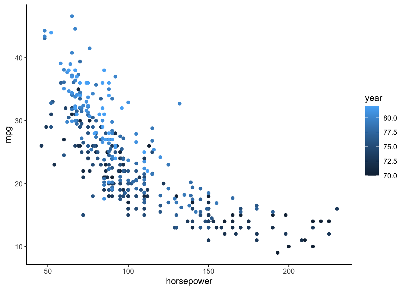
  dplyr::select(mpg, horsepower, year)

Let’s use the cars data to compare three linear regression models of fuel efficiency in miles per gallon (mpg) by engine power (horsepower):

# Raw data
cars_plot <- ggplot(cars, aes(x = horsepower, y = mpg)) + 
  geom_point()
cars_plot

# model 1: 1 predictor (y = b0 + b1 x)
cars_plot + 
  geom_smooth(method = "lm", se = FALSE)

# model 2: 2 predictors (y = b0 + b1 x + b2 x^2)
cars_plot + 
  geom_smooth(method = "lm", se = FALSE, formula = y ~ poly(x, 2))

# model 3: 19 predictors (y = b0 + b1 x + b2 x^2 + ... + b19 x^19)
cars_plot + 
  geom_smooth(method = "lm", se = FALSE, formula = y ~ poly(x, 19))

Goal

Let’s evaluate and compare these models by training and testing them using different data.

155 review: set.seed()

Run the two chunks below multiple times each. Afterward, summarize what set.seed() does and why it’s important to being able to reproduce a random sample.

sample_n(cars, 2)

set.seed(253)
sample_n(cars, 2)

Solution

set.seed() is used to create the same “random numbers” each time a random function is called.

Note that is if you want to get exactly the same random result, set.seed() needs to be run right before the call to random function, every time.

It is important so that you can reproduce the same random sample every time you knit your work.

There might be different results across computers/platforms as they might be using different pseudo-random number generators. The most important thing is for your code to be consistent.

Training and test sets

Let’s randomly split our original 392 sample cars into two separate pieces: select 80% of the cars to train (build) the model and the other 20% to test (evaluate) the model.

# Set the random number seed
set.seed(8)
    
# Split the cars data into 80% / 20%
# Ensure that the sub-samples are similar with respect to mpg
cars_split <- initial_split(cars, strata = mpg, prop = 0.8)

# Check it out
# What do these numbers mean?
cars_split

# Get the training data from the split
cars_train <- cars_split %>% 
  training()
    
# Get the testing data from the split
cars_test <- cars_split %>% 
  testing()

# The original data has 392 cars
nrow(cars)
    
# How many cars are in cars_train?
    
# How many cars are in cars_test?

Solution

# Set the random number seed
set.seed(8)

# Split the cars data into 80% / 20%
# Ensure that the sub-samples are similar with respect to mpg
cars_split <- initial_split(cars, strata = mpg, prop = 0.8)
cars_split

## <Training/Testing/Total>
## <312/80/392>

# Get the training data from the split
cars_train <- cars_split %>% 
  training()

# Get the testing data from the split
cars_test <- cars_split %>% 
  testing()

# The original data has 392 cars
nrow(cars)

## [1] 392

# How many cars are in cars_train?
nrow(cars_train)

## [1] 312

# How many cars are in cars_test?
nrow(cars_test)

## [1] 80

Reflect on the above code

Why do we want the training and testing data to be similar with respect to mpg (strata = mpg)? What if they weren’t?
Why did we need all this new code instead of just using the first 80% of cars in the sample for training and the last 20% for testing?

Solution

Suppose, for example, the training cars all had higher mpg than the test cars. Then the training model likely would not perform well on the test cars, thus we’d get an overly pessimistic measure of model quality.
If the cars are ordered in some way (eg: from biggest to smallest) then our training and testing samples would have systematically different properties.

Build the training model

# STEP 1: model specification
lm_spec <- linear_reg() %>% 
  set_mode("regression") %>% 
  set_engine("lm")

# STEP 2: model estimation using the training data
# Construct the 19th order polynomial model using the TRAINING data
model_19_train <- ___ %>% 
  ___(mpg ~ poly(horsepower, 19), data = ___)

Solution

# STEP 1: model specification
lm_spec <- linear_reg() %>% 
set_mode("regression") %>% 
set_engine("lm")

# STEP 2: model estimation using the training data
# Construct the 19th order polynomial model using the TRAINING data
model_19_train <- lm_spec %>% 
fit(mpg ~ poly(horsepower, 19), data = cars_train)

Evaluate the training model

# How well does the TRAINING model predict the TRAINING data?
# Calculate the training (in-sample) MAE
model_19_train %>% 
  augment(new_data = ___) %>% 
  mae(truth = mpg, estimate = .pred)

# How well does the TRAINING model predict the TEST data?
# Calculate the test MAE
model_19_train %>% 
  augment(new_data = ___) %>% 
  mae(truth = mpg, estimate = .pred)

Solution

# How well does the training model predict the training data?
# Calculate the training (in-sample) MAE
model_19_train %>% 
augment(new_data = cars_train) %>% 
mae(truth = mpg, estimate = .pred)

## # A tibble: 1 × 3
##   .metric .estimator .estimate
##   <chr>   <chr>          <dbl>
## 1 mae     standard        2.99

# How well does the training model predict the test data?
# Calculate the test MAE
model_19_train %>% 
augment(new_data = cars_test) %>% 
mae(truth = mpg, estimate = .pred)

## # A tibble: 1 × 3
##   .metric .estimator .estimate
##   <chr>   <chr>          <dbl>
## 1 mae     standard        6.59

Punchline
The table below summarizes your results for train_model_19 as well as the other two models of interest. (You should confirm the other two model results outside of class!)

Model	Training MAE	Testing MAE
`mpg ~ horsepower`	3.78	4.00
`mpg ~ poly(horsepower, 2)`	3.20	3.49
`mpg ~ poly(horsepower, 19)`	2.99	6.59

Answer the following and reflect on why each answer makes sense:

Within each model, how do the training errors compare to the testing errors? (This isn’t always the case, but is common.)
Why about the training and test errors for the third model suggest that it is overfit to our sample data?
Which model seems the best with respect to the training errors?
Which model is the best with respect to the testing errors?
Which model would you choose?

Solution

the training errors are smaller
the test MAE is much larger than the training MAE
the 19th order polynomial
the quadratic
the quadratic

Code for the curious

I wrote a function calculate_MAE() to automate the calculations in the table. If you’re curious, pick through this code!

# Write function to calculate MAEs
calculate_MAE <- function(poly_order){
  # Construct a training model
  model <- lm_spec %>% 
    fit(mpg ~ poly(horsepower, poly_order), cars_train)
  
  # Calculate the training MAE
  train_it <- model %>% 
    augment(new_data = cars_train) %>% 
    mae(truth = mpg, estimate = .pred)
      
  # Calculate the testing MAE
  test_it <- model %>% 
    augment(new_data = cars_test) %>% 
    mae(truth = mpg, estimate = .pred)
      
  # Return the results
  return(data.frame(train_MAE = train_it$.estimate, test_MAE = test_it$.estimate))
}
    
# Calculate training and testing MSEs
calculate_MAE(poly_order = 1)

##   train_MAE test_MAE
## 1  3.779331 4.004333

calculate_MAE(poly_order = 2)

##   train_MAE test_MAE
## 1  3.199882 3.487022

calculate_MAE(poly_order = 19)

##   train_MAE test_MAE
## 1  2.989305 6.592341

# For those of you interested in trying all orders...

results <- purrr::map_df(1:19,calculate_MAE) %>% 
  mutate(order = 1:19) %>%
  pivot_longer(cols=1:2,names_to='Metric',values_to = 'MAE') 

results %>%
  ggplot(aes(x = order, y = MAE, color = Metric)) + 
  geom_line() + 
  geom_point(data = results %>% filter(Metric == 'test_MAE') %>% slice_min(MAE)) + 
  geom_point(data = results %>% filter(Metric == 'train_MAE') %>% slice_min(MAE))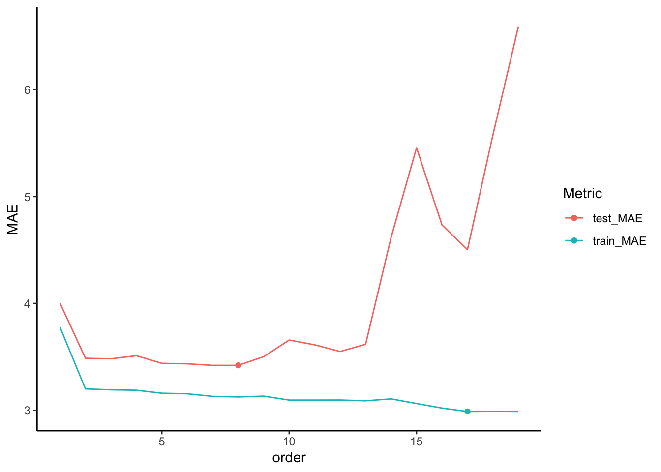

Final reflection
1. The training / testing procedure provided a more honest evaluation and comparison of our model predictions. How might we improve upon this procedure? What problems can you anticipate in splitting our data into 80% / 20%?
2. Summarize the key themes from today in your own words.

Solution

This will be discussed in the next video!

STAT 155 REVIEW: data drill

Construct and interpret a plot of mpg vs horsepower and year.
Calculate the average mpg.
Calculate the average mpg for each year. HINT: group_by()
Plot the average mpg by year.

Solution

# a. One of many options
ggplot(cars, aes(x = horsepower, y = mpg, color = year)) + 
  geom_point()

# b
cars %>% 
summarize(mean(mpg))

##   mean(mpg)
## 1  23.44592

# c
cars %>% 
  group_by(year) %>% 
  summarize(mean_mpg = mean(mpg))

## # A tibble: 13 × 2
##     year mean_mpg
##    <dbl>    <dbl>
##  1    70     17.7
##  2    71     21.1
##  3    72     18.7
##  4    73     17.1
##  5    74     22.8
##  6    75     20.3
##  7    76     21.6
##  8    77     23.4
##  9    78     24.1
## 10    79     25.1
## 11    80     33.8
## 12    81     30.2
## 13    82     32

# d
cars %>% 
  group_by(year) %>% 
  summarize(mean_mpg = mean(mpg)) %>% 
  ggplot(aes(y = mean_mpg, x = year)) + 
  geom_point()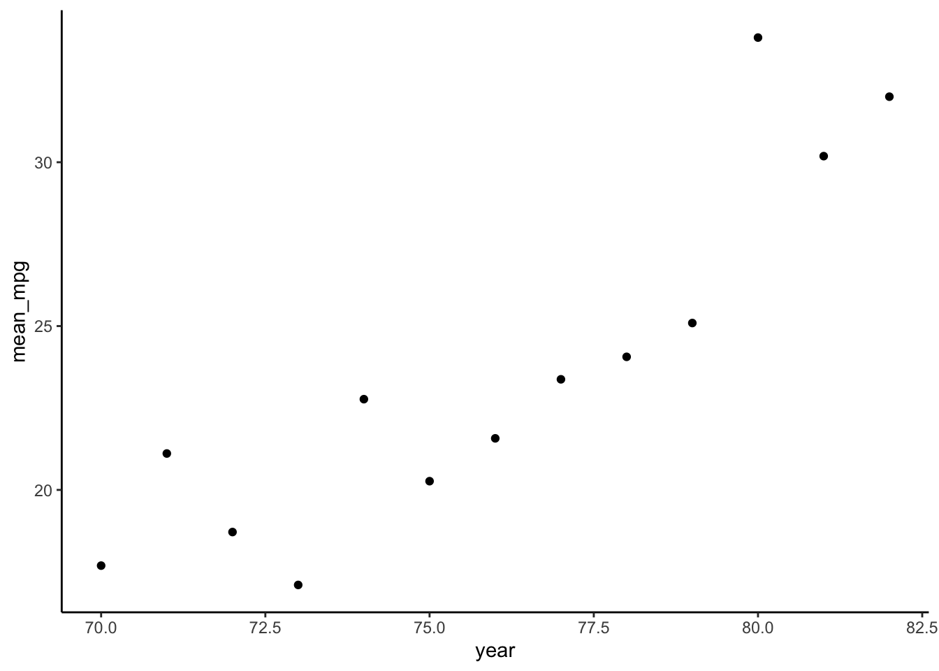

Digging deeper (optional)

Check out the online solutions for exercise 6. Instead of calculating MAE from scratch for 3 different models, I wrote a function calculate_MAE() to automate the process. After picking through this code, adapt the function so that it also returns the \(R^2\) value of each model.

Done!

Knit your notes.
Check the solutions in the course website.
If you finish all that during class, start on Homework 2!