1 Introductions & Overview

Settling In

Welcome to Correlated Data!

Sit with a group of 3-4 people that you do not know well.

Introduce yourself

Name, pronounciation tips, pronouns
Macalester connections (e.g., majors/minors/concentrations, clubs, teams, events regularly attended)
How are you feeling about the coming semester?
One thing from break that you are proud of!
If you could use data to investigate anything, what would it be and why?

Get out a notebook to take notes for the class. I recommend:

Before Class Notes: on readings/videos; make notes of questions that you have.
In Class Notes: concepts, statistical proofs, models (pros/cons, theory, and implementation in R)

Everything on the slides is in the online manual: https://bcheggeseth.github.io/452_fall_2025/

Plan for today

Introductions
Foundational Ideas
Course Logistics
Small Group Activity

Introductions

Instructor

Who I am

Prof. Brianna Heggeseth (she/her)

[bree-AH-na] (Anna like in Frozen) [HEG-eh-seth]

https://bcheggeseth.github.io

Where I’ve been

Students

Directions:

You’ll spend about 10 minutes in small groups.

. . .

When we come back together, I’m going to ask everyone to take a turn and do the following:

Introduce one of your small group mates.
Share one insight/idea from your discussion about learning & AI experiences / grades.

. . .

So take a moment to:

Introduce yourselves (if you didn’t get a chance already) in whatever way you feel appropriate (e.g. name, pronouns, majors/minors, how you’re feeling about the semester, things you’re looking forward to, moment of pride from break).
Discuss the following:
- What are some things that have contributed to positive learning experiences in your courses that you would like to have in place for this course? What has contributed to negative experiences that you would like to prevent?
- What is your experience with Generative AI? Positives? Negatives?
- What has been the role of grades in your learning?
- What if we got rid of grades? Pros? Cons on your learning?

Now, take a moment to introduce the person to your left to the rest of the class. Share:

their name (take time to ensure you pronounced it correctly) and
one thing you learned about them.

Learning Goals

Explain the similarities and differences between time series, longitudinal, and spatial data.
Explain why and how standard methods such as linear regression (estimated by ordinary least squares abbreviated as OLS) fail on correlated data.
Be comfortable with working with time/date data using the lubridate R package.
Further develop your comfort playing with and manipulating data in R.

Foundational Ideas

More information found in our notes https://mac-stat.github.io/CorrelatedDataNotes/

Correlated Data

Correlated Data: Data observations that are not independent by design.

Information contained in one data point overlaps with information in another data point.
Standard measures of uncertainty (standard errors) will be wrong.
Total amount of information cannot be solely captured with the sample size.

. . .

Data Examples

If you collect data on siblings, the children with similar genetics and the same home environment will be more similar to each other than randomly selected children.
Students who are in the same classroom will be more similar in their learning than students from different classrooms because they have a common teacher and curriculum.
Data collected on the same individuals over time; the repeated measurements on an individual will be more similar than measurements across different individuals.
Air pollution measurements will be more similar to each other if they are taken closer in space (100 feet apart as compared to 5 miles apart).

. . .

In this class, we’ll talk about three correlated data types.

Time Series Data (temporal data)
Longitudinal Data (temporal data)
Spatial Data

. . .

Overall: Observations measured closer in time or space should be more similar (more positively correlated) than observations measured further away in time or space.

Time Series Data

We call temporal data a time series if we have measurements

for a small number of units or subjects
taken at regular and equally-spaced times (often more than 20 times).

Longitudinal Data

We call temporal data longitudinal data if we have measurements

for many units or subjects
taken approximately 2 to 20 observations times
at typically irregular, unequally-spaced times, which may differ between subjects.

Spatial Data

Spatial data can be measured

as observations at a point in space, typically measured using longitude and latitude, or
as areal units which are aggregated summaries based on natural or societal boundaries such as county districts, census tracts, postal code areas, or any other arbitrary spatial partition.

Course Logistics

Structure

Before Class:

Watch videos / read sections of course notes (see Schedule on Course Website)
Take notes on video / reading
Ask questions in office hours

. . .

During Class:

In community and collaboration,

Reinforce and develop understanding about concepts
Practice communicating with probability notation
Implement in R
Contribute to a positive learning environment

. . .

After Class:

Work on homework & projects
Reflect on your understanding and engagement
Rewrite / revise your notes
Ask questions in office hours

Assignments & Assessments

Self & Peer Feedback

In-class Activities & Solutions

. . .

Instructor Qualitative Feedback

Homeworks due at class time (extensions of in-class activities or progressing on mini project)
Content Conversations

. . .

Instructor Assessment

Three mini projects
Capstone projects

. . .

Self Reflection & Assessment

Monthly reflections about your learning
Final self assessment & reflection

Navigating Materials

Navigate to the syllabus section of our course site.

Navigate to the Moodle site of our course site.

Small Group Activity

In this course, we will spend time with real data as well as the theory of the statistical models and methods that we use for correlated data.

. . .

The first half of the semester will be theory-heavy so that we can establish some important theoretical threads that we will weave through the different types of correlated data.

. . .

So today, we work with real, correlated data and start thinking about how we may plot temporal data (data collected over time) using standard methods and trying to come up with creative ways to explore this data.

Playing with Correlated Data

Download a template Qmd file to start from here.
Each of you should work on your own Qmd file, but you need to check in with each other on each question. Help each other. Share ideas and insight.
Open RStudio and the template file. Make sure you have installed the R packages you need for today.

We will be using the tidyverse and lubridate package today. If you have not seen these packages yet, I recommend checking out the data transformation and visualization cheatsheets (https://www.rstudio.com/resources/cheatsheets/). The symbol %>% is a pipe and it passes whatever is to the left as the first argument to the function on the right.

#Run this R chunk first!
library(tidyverse)
library(lubridate) #install.packages('lubridate') if needed

#options(gargle_oob_default = TRUE) #run if you are working on Mac RStudio Server

Data Context: Temperatures & Energy Use

Minnesota winters are cold. In St. Paul, homes and apartments are typically 50 to 100 years old or older. This means they may not be energy efficient in that they may be drafty and without modern insulation.

To learn about energy use in a St. Paul home, Prof. Heggeseth’s family installed a Nest thermostat in the Dining Room in Jan 2019 to control the heat and record the temperature and energy use in their home (built in 1914). They installed another Nest thermostat Upstairs in July 2019 to control the air conditioning (cooling). Then in Fall 2019, they redid their heating system to have three zones and added a Basement thermostat. You have access to almost a full year of data in 2019.

Part of this exercise is to consider and engage with the Data Generating Process, the entire process by which data values came to be and how the values were measured/recorded/stored. Some factors in this process will be random and others are determinist.

To figure out the Data Generating Process,

Learn about the system/context that you are studying
Ask questions
- Explore the data to see if the answer is in the data itself
- If the data can’t answer the question, ask the person who collected the data.

Exercises

Today, we are going to explore real data that are continuously being collected, every five to ten minutes, and stored in a Google spreadsheet. With the code below, we read in the data stored in Google Sheets.

library(tidyverse)
nest  <- read_csv("https://docs.google.com/spreadsheets/d/e/2PACX-1vQnSHPcthKoRmgCOgoW-Sl_vRRm2mUTKhKIYW04OQqOAste8lGLI71fq3WQIvtC4C8PBdSNfnw21PB1/pub?output=csv")

Check out the variables in the data set. Note that Location1, Location2, Location3 are not going to be useful variables for us; they are constant, so I remove them with the code below.

nest <- nest %>%
  select(-Location1,-Location2,-Location3)

head(nest) #prints first 6 rows of data frame
names(nest)

List the variables and their type (categorical, continuous) and guess what they measure.

Before we go any further, I want to introduce you to a package that will be very useful for you especially if we have variables of dates or time. The lubridate package! The documentation for the package is here: https://lubridate.tidyverse.org/

nest <- nest %>%
  mutate(Date = mdy_hms(Date)) %>% # convert character string to date/time object
  mutate(DateTime = force_tz(Date, "America/Chicago")) %>% #force the time zone to be Central Time
  mutate(DateOnly = date(DateTime)) #pull out the date only

Use the lubridate functions hour() and minute() within mutate() to create new variables for the hour in a day and minutes within the hour. Create a quantitative, continuous variable in the nest dataset called Time, that combines the hour and minute with decimal values of 9.5 to represent 9:30am and 21.5 to represent 9:30pm, for example.

#mutate adds variables to the data set
nest <- nest %>%
  mutate() %>%  #start with Hour and Minute
  mutate() #then do Time

Use the lubridate functions day() and month() to create new variables for day within the month and the month within the year. Create a quantitative variable in the nest dataset, called MonthDay, that combines the month and day such that April 15 is 4.5, for example. Hint: days_in_month() will be useful to do this.

Create a categorical variable called DayofWeeek with weekdays labels using wday(). Use ?wday to look at documentation and look at labels.

Create a line plot (geom_line) with DateTime and DiningTemp. Comment on what patterns you notice, what you learn and questions you have about the data.

Create a line plot (geom_line) with Time and DiningTemp, grouped by MonthDay, colored by the DayofWeek, and faceted by Month. Comment on what patterns you notice, what you learn and questions you have.

Create a scatterplot (geom_jitter) of DiningTemp with the DiningPrevTemp (temperature 5 or 10 minutes previously). Do the same for the observation 10-20 minutes previously. Comment on what patterns you notice, what you learn and questions you have.

nest <- nest %>%
  mutate(DiningPrevTemp = lag(DiningTemp), DiningPrevTemp2 = lag(DiningTemp, 2), DiningPrevTemp3 = lag(DiningTemp, 3))

Create a tile plot (geom_tile) of Time against MonthDay filled by DiningMode, but only for the observations between February and May. Ensure the width of the tile corresponds to 10 minute intervals. Try to ensure that you can read Month from top to bottom and time from left to right. Comment on what you patterns notice, what you learn and questions you have.

Explore the relationship between outside temperature and the heating and cooling systems. Create plots with short summaries of the insights you gain about the energy efficiency of our home, the schedule of our thermostat, etc. Be creative. Think outside the box. Come up with an idea of what you want to plot and ask for help with coding questions.

Some ideas to get you started: summarize each day by the proportion of time the heater was on (or longest/shortest stretch of time with no heat or the max/min difference between Target Temp and Actual Temp) as well as summaries of temperature (min, mean, median, max).

Solutions

Small Group Activity

Solution

Date: continuous date and time
____TargetTemp: Continuous target temperature of ____ Room in Farenheit
____Temp: Continuous actual temperature of Dining Room in Farenheit
____Humidity: Continuous actual humidity of Dining Room in percent
____Mode: Categorical mode (heat, off, cool)
OutTemp: Continuous outside temperature in Farenheit
OutHumidity: Continuous outside humidity in percent

Solution

#mutate adds variables to the data set
nest <- nest %>%
  mutate(Hour = hour(Date), Minute = minute(Date)) %>%  #start with Hour and Minute
  mutate(Time = Hour + Minute/60) #then do Time

head(nest)

# A tibble: 6 × 20
  Date                DiningTargetTemp DiningTemp DiningHumidity DiningMode
  <dttm>                         <dbl>      <dbl>          <dbl> <chr>     
1 2019-01-18 19:46:23               68         67             20 heating   
2 2019-01-18 19:49:20               68         67             20 heating   
3 2019-01-18 19:52:08               67         67             20 off       
4 2019-01-18 19:54:19               67         67             20 off       
5 2019-01-18 19:59:19               67         67             20 off       
6 2019-01-18 20:04:19               67         67             20 off       
# ℹ 15 more variables: UpstairsTargetTemp <dbl>, UpstairsTemp <dbl>,
#   UpstairsHumidity <dbl>, UpstairsMode <chr>, BasementTargetTemp <dbl>,
#   BasementTemp <dbl>, BasementHumidity <dbl>, BasementMode <chr>,
#   OutTemp <dbl>, OutHumidity <dbl>, DateTime <dttm>, DateOnly <date>,
#   Hour <int>, Minute <int>, Time <dbl>

Solution

#mutate adds variables to the data set
nest <- nest %>%
  mutate(Month = month(Date), Day = day(Date)) %>%
  mutate(MonthDay = Month + Day/days_in_month(Date))

Solution

#mutate adds variables to the data set
nest <- nest %>%
  mutate(DayofWeek = wday(Date, label = TRUE))

Solution

nest %>%
  ggplot(aes(x = DateTime, y = DiningTemp)) + 
  geom_line() +
  geom_vline(xintercept = nest %>% filter(!is.na(UpstairsMode)) %>% slice_min(DateTime) %>% pull(DateTime), color = 'red') +
  geom_vline(xintercept = nest %>% filter(!is.na(BasementMode)) %>% slice_min(DateTime) %>% pull(DateTime), color = 'blue')

Notes

More variability in the winter
Highest temperatures occurred when on vacation in around 4th of July
Dynamics shift when Upstairs thermostat installed and when Basement thermostat installed (split into 3 zones)
Data Context and Data Generation Mechanism is vital to know! Sometimes the data can’t tell the whole story.

Solution

nest %>%
  ggplot(aes(x = Time, y = DiningTemp, group = MonthDay, color = DayofWeek)) + 
  geom_line() + 
  facet_wrap(~ Month)

Notes

More variability in the winter
Very different within day patterns by month, depending on outside temperature / season.

Solution

nest <- nest %>%
  mutate(DiningPrevTemp = lag(DiningTemp), DiningPrevTemp2 = lag(DiningTemp, 2), DiningPrevTemp3 = lag(DiningTemp, 3)) 

nest %>%
  ggplot(aes(x = DiningPrevTemp, y = DiningTemp)) +
  geom_jitter()

nest %>%
  ggplot(aes(x = DiningPrevTemp2, y = DiningTemp)) +
  geom_jitter()

nest %>%
  ggplot(aes(x = DiningPrevTemp3, y = DiningTemp)) +
  geom_jitter()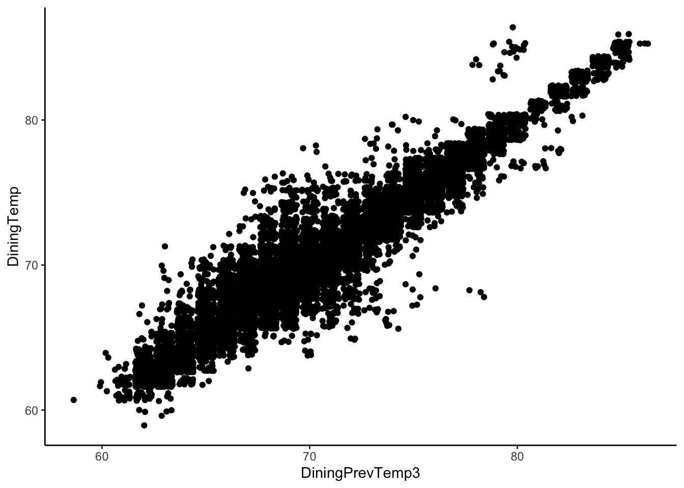

Notes

Temperatures within 5 minutes of each are highly correlated
The correlation decreases in magnitude as the time between observations increases

Solution

nest %>%
  filter(Month >= 2, Month <= 5) %>%
  ggplot(aes(x = Time, y = MonthDay, fill = DiningMode)) +
  geom_tile(width = 10/60) +
  scale_y_reverse()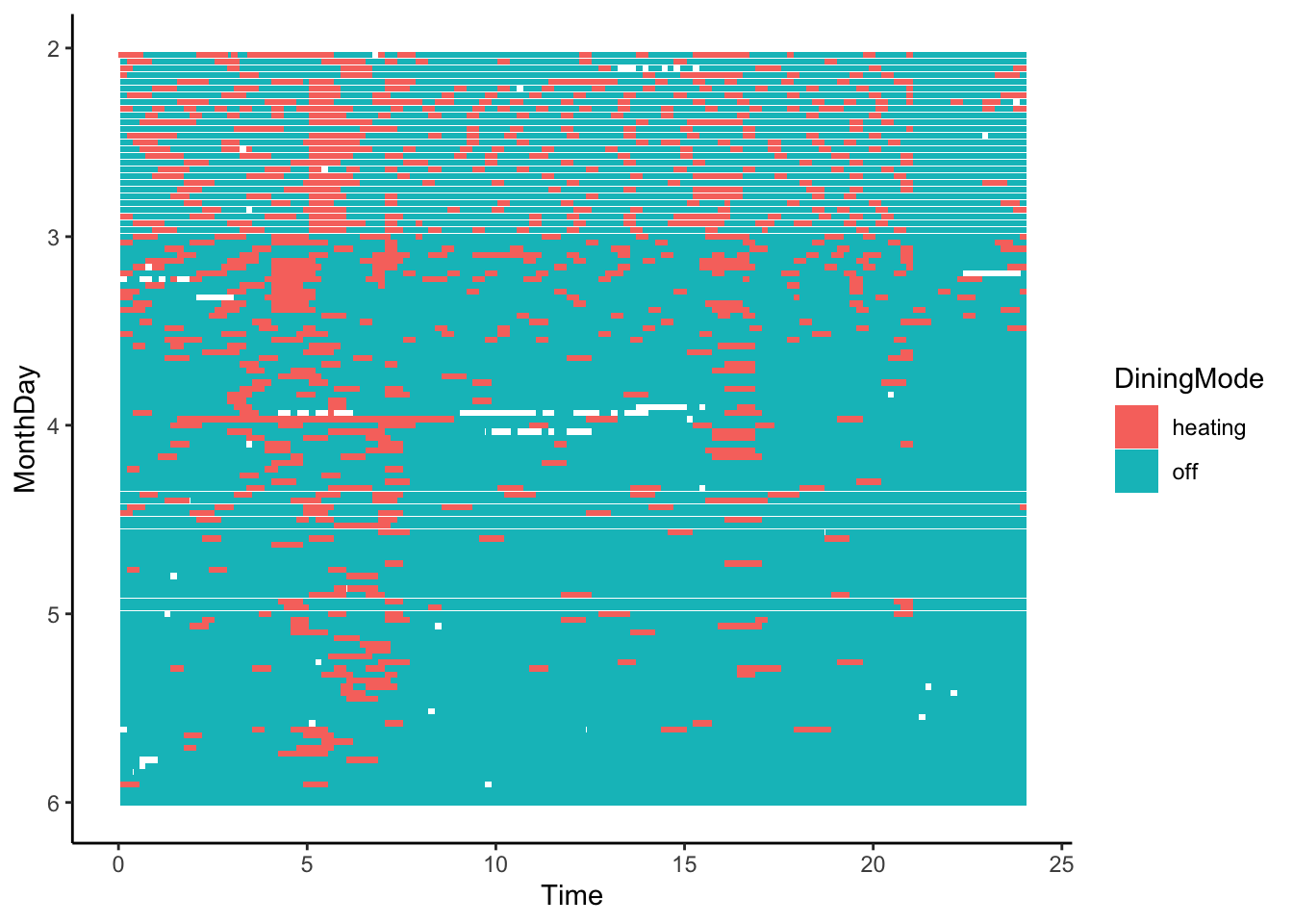

Solution

Many potential solutions here.

Date1 <- nest %>% filter(!is.na(UpstairsMode)) %>% slice_min(DateTime) %>% pull(DateTime)
Date2 <- nest %>% filter(!is.na(BasementMode)) %>% slice_min(DateTime) %>% pull(DateTime)

nest_by_day <- nest %>%
  group_by(MonthDay) %>%
  summarize(PropHeat = sum(DiningMode == 'heating')/n(),
            PropHeat_morning = sum(DiningMode[Time < 6] == 'heating')/sum(!is.na(DiningMode[ Time < 6])),
            PropHeat_day = sum(DiningMode[Time < 20 & Time > 6] == 'heating')/sum(!is.na(DiningMode[Time < 20 & Time > 6])),
            PropHeat_evening = sum(DiningMode[Time > 20] == 'heating')/sum(!is.na(DiningMode[ Time > 20])),
            OutTemp_Min = min(OutTemp,na.rm=TRUE), 
            OutTemp_Max = max(OutTemp,na.rm=TRUE), 
            OutTemp_9am = mean(OutTemp[Time >= 9 & Time <= 9 + 11/60],na.rm = TRUE),
            OutTemp_3pm = mean(OutTemp[Time >= 15 & Time <= 15 + 11/60],na.rm = TRUE),
            System = case_when(min(DateOnly) < Date1 ~ 'Dining Only',
                               min(DateOnly) < Date2 ~ 'Dining + Upstairs Air',
                               TRUE ~ 'Basement Zone Included'))
  

nest_by_day %>%
  ggplot(aes(x = OutTemp_Min, y = PropHeat)) + 
  geom_point() +
  geom_vline(xintercept = 51)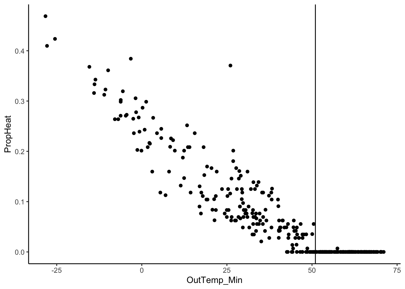

nest_by_day %>%
  ggplot(aes(x = OutTemp_3pm, y = PropHeat)) + 
  geom_point()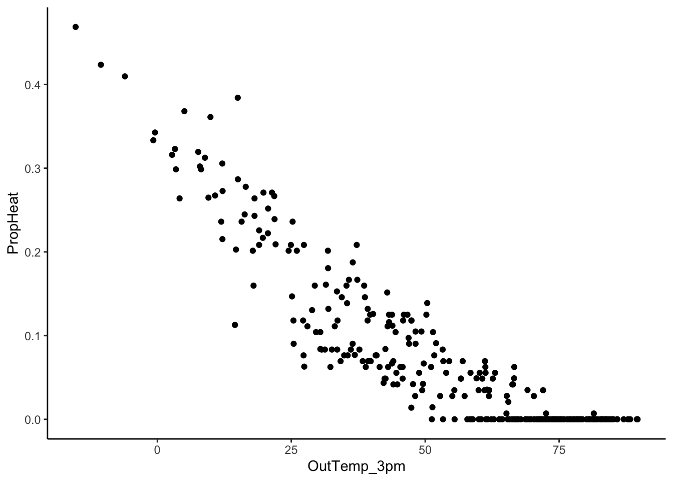

nest_by_day %>%
  mutate(NoHeat = PropHeat < 0.01) %>%
  ggplot(aes(x = OutTemp_Min, y = OutTemp_3pm, color = NoHeat)) + 
  geom_point() +
  geom_vline(xintercept = c(42,51))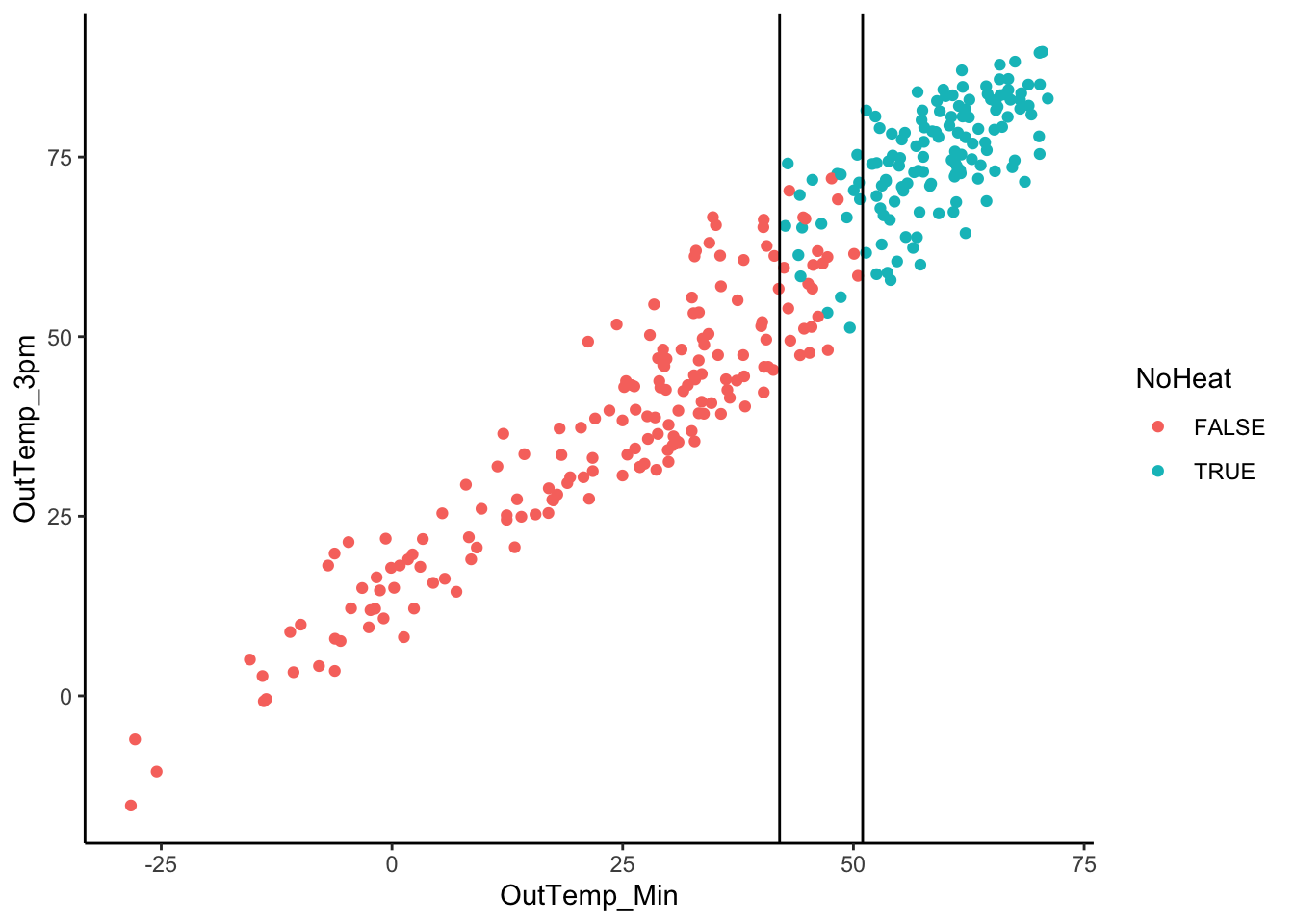

nest_by_day %>%
  mutate(NoHeat = PropHeat < 0.01, Month = floor(MonthDay)) %>%
  ggplot(aes(x = OutTemp_9am, y = OutTemp_3pm, shape = NoHeat, color = System)) + 
  geom_point()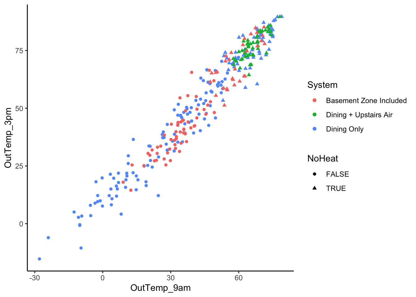

nest_by_day %>%
  mutate(NoHeat = PropHeat < 0.01, Month = floor(MonthDay)) %>%
  filter(NoHeat == FALSE, OutTemp_9am > 51)

# A tibble: 10 × 12
   MonthDay PropHeat PropHeat_morning PropHeat_day PropHeat_evening OutTemp_Min
      <dbl>    <dbl>            <dbl>        <dbl>            <dbl>       <dbl>
 1     4.23   0.0486           0.111        0.0357                0        45.6
 2     4.8    0.0350           0            0.0595                0        48.3
 3     5.13   0.0278           0.0556       0.0238                0        43.0
 4     5.16   0.0347           0            0.0595                0        47.2
 5     5.35   0.0486           0            0.0833                0        40.6
 6     5.42   0.0280           0.0278       0.0357                0        40.2
 7     5.45   0.0347           0            0.0595                0        47.6
 8     5.68   0.0347           0.111        0.0119                0        45.6
 9     5.74   0.0556           0.222        0                     0        50.5
10     5.77   0.0355           0            0.0595                0        50.1
# ℹ 6 more variables: OutTemp_Max <dbl>, OutTemp_9am <dbl>, OutTemp_3pm <dbl>,
#   System <chr>, NoHeat <lgl>, Month <dbl>

nest_by_day %>%
  mutate(NoHeat = PropHeat < 0.01, Month = floor(MonthDay)) %>%
  filter(!NoHeat, PropHeat_morning >= 0.01) %>%
  ggplot(aes(x = OutTemp_9am, y = PropHeat_morning, color = System)) + 
  geom_point() +
  geom_smooth(se = FALSE) +
  geom_smooth(method = 'lm', se = FALSE)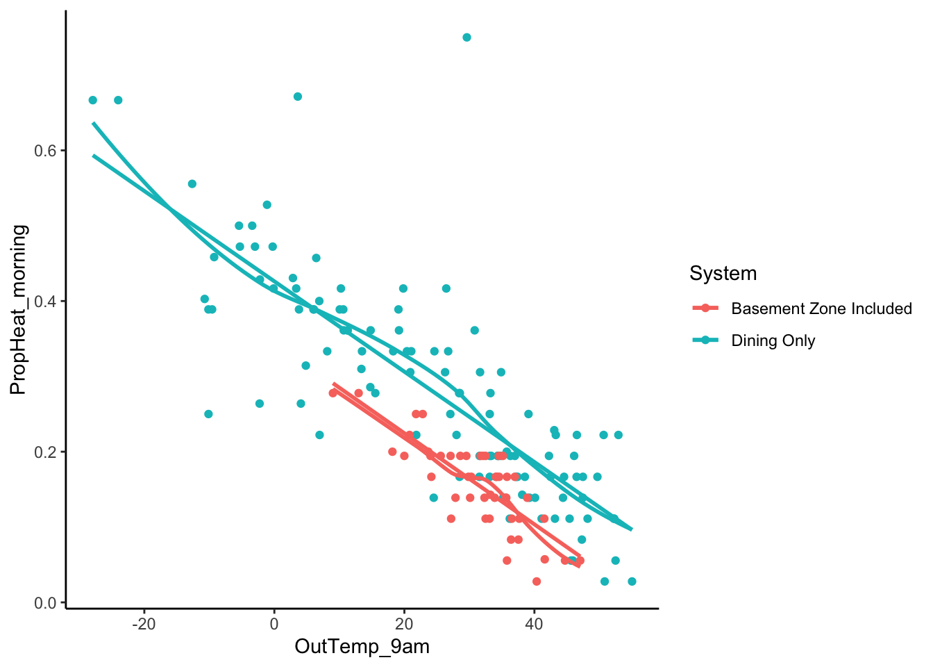

nest_by_day %>%  mutate(NoHeat = PropHeat < 0.01, Month = floor(MonthDay)) %>%
  filter(!NoHeat, PropHeat_day >= 0.01) %>%
  ggplot(aes(x = OutTemp_3pm, y = PropHeat_day, color = System)) + 
  geom_point() +
  geom_smooth(se = FALSE) +
  geom_smooth(method = 'lm', se = FALSE)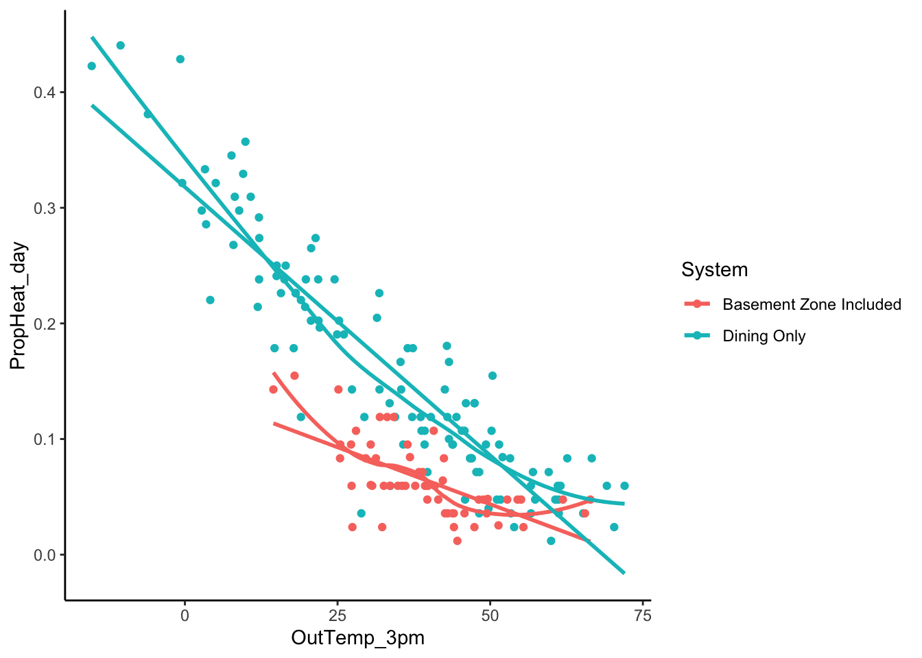

Wrap-Up

Finishing the Activity

If you didn’t finish the activity, no problem! Be sure to complete the activity outside of class, review the solutions in the online manual, and ask any questions on Slack or in office hours.
Re-organize and review your notes to help deepen your understanding, solidify your learning, and make homework go more smoothly!

After Class

Before the next class, please do the following:

Set up the software and systems we need following these instructions.
Update your Slack profile with preferred name, pronouns, name pronunciation. (To find your profile, click on your name under Direct Messages on the left menu, and click “Edit Profile”.)
Complete the pre-course information gathering survey.
Complete HW0 on Moodle.
Take a look at the Schedule page to see how to prepare for the next class.