Covariance is a function of difference (direction + distance) in time/space
For spatial data, isotropy is a stronger assumption: covariance is a function of distance only
Intrinsic Stationarity
Variance of difference depends only on difference in time/space
These constraints allow us to estimate variance and covariance with limited data.
Learning Goals
Explain the differences between model components such as trend, seasonality, serial error, and measurement error.
Understand and implement the tools available to model and remove trends (polynomials, splines, local regression, moving average filters, differencing) and seasonality (indicators, sine and cosine curves, seasonality differencing)
Notes: Model Components
Components
For the Data Generating Process, we may model it as
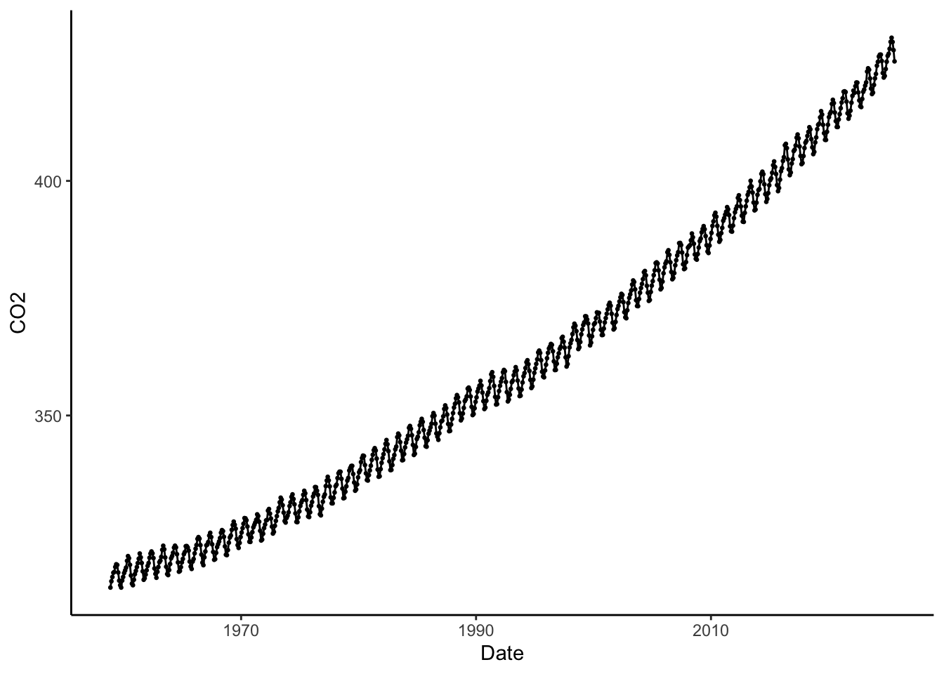
The data come from Mauna Loa Observatory (MLO) in Hawaii. According to the website, “the undisturbed air, remote location, and minimal influences of vegetation and human activity at MLO are ideal for monitoring constituents in the atmosphere that can cause climate change.”
You’ll analyze the CO2 concentration measurements available on the MLO’s website. CO2 measurements have been collected since 1958 until present day and they are presented as monthly averages. Click the website below to see the data in the text file. The first 50 lines include information about the data and provide variable definitions. Read the data into R with the code below. I have provided you some code to add Variable Names to a data frame.
co2 <-read.table('ftp://aftp.cmdl.noaa.gov/products/trends/co2/co2_mm_mlo.txt',skip=50,header=FALSE)names(co2) <-c('Year','Month','Date','CO2','CO2Trend','Days','sdDays','seCO2')co2[co2 <0] <-NAhead(co2)
  Year Month     Date    CO2 CO2Trend Days sdDays seCO2
1 1958    11 1958.874 313.33   315.21   NA     NA    NA
2 1958    12 1958.956 314.67   315.43   NA     NA    NA
3 1959     1 1959.041 315.58   315.52   NA     NA    NA
4 1959     2 1959.126 316.49   315.84   NA     NA    NA
5 1959     3 1959.203 316.65   315.37   NA     NA    NA
6 1959     4 1959.288 317.72   315.42   NA     NA    NA
Exercises
Using ggplot(), make a plot of the CO2 concentration (CO2) as a function of the Date. Comment on what you observe in the data context.
require(ggplot2)require(dplyr)
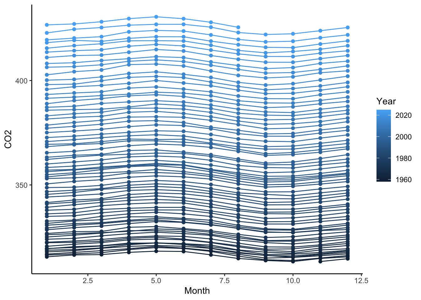
Using ggplot(), make a plot of the CO2 concentration (CO2) as a function of the Month, grouped by Year. Comment on what you observe in the data context.
Estimating Trend
Estimate the trend of the data using a moving average filter. Create a vector of weights (save it as fltr) for points before and after the time that you are estimating the trend, such that you are adequately averaging over one years of data.
# Save data as a ts (time series) object to keep track of time and the values.co2_ts_data <-ts(co2$CO2, start =c(1958,11), frequency =12)
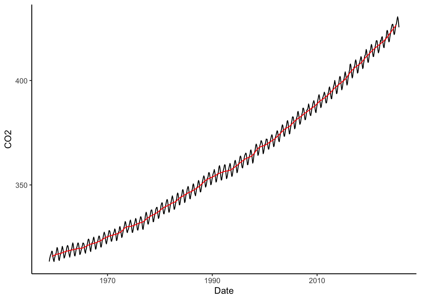
fltr <- ?? #vector of weights for moving average filter# Adjust data frame by adding MA trend as variable co2 <- co2 %>%mutate( co2Trend_MA =as.numeric(stats::filter(co2_ts_data, filter = fltr, method ='convo', sides =2)))co2 %>%ggplot(aes(x = Date, y = CO2)) +geom_line() +geom_line(aes(y = co2Trend_MA), color ='red') +theme_classic()
Estimate the trend of the data using local regression, loess(). Adjust span= so as to only capture the trend and not the seasonality. Compare the estimated trend with that from the moving average.
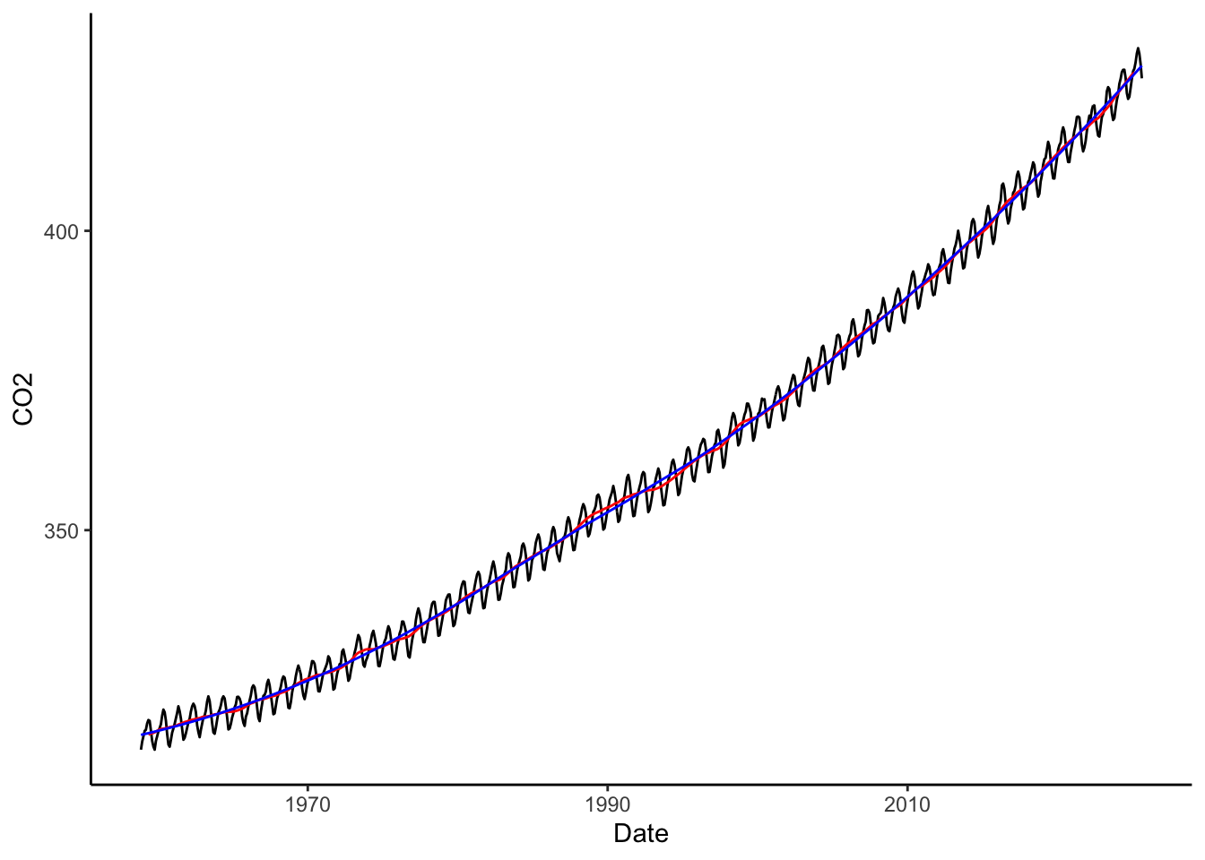
# Adjust data frame by adding Loess trend as variable co2 <- co2 %>%mutate(co2Trend_loess =predict(loess(CO2 ~ Date, data = co2, span = ??)))co2 %>%ggplot(aes(x = Date, y = CO2)) +geom_line() +geom_line(aes(y = co2Trend_MA), color ='red') +geom_line(aes(y = co2Trend_loess), color ='blue') +theme_classic()
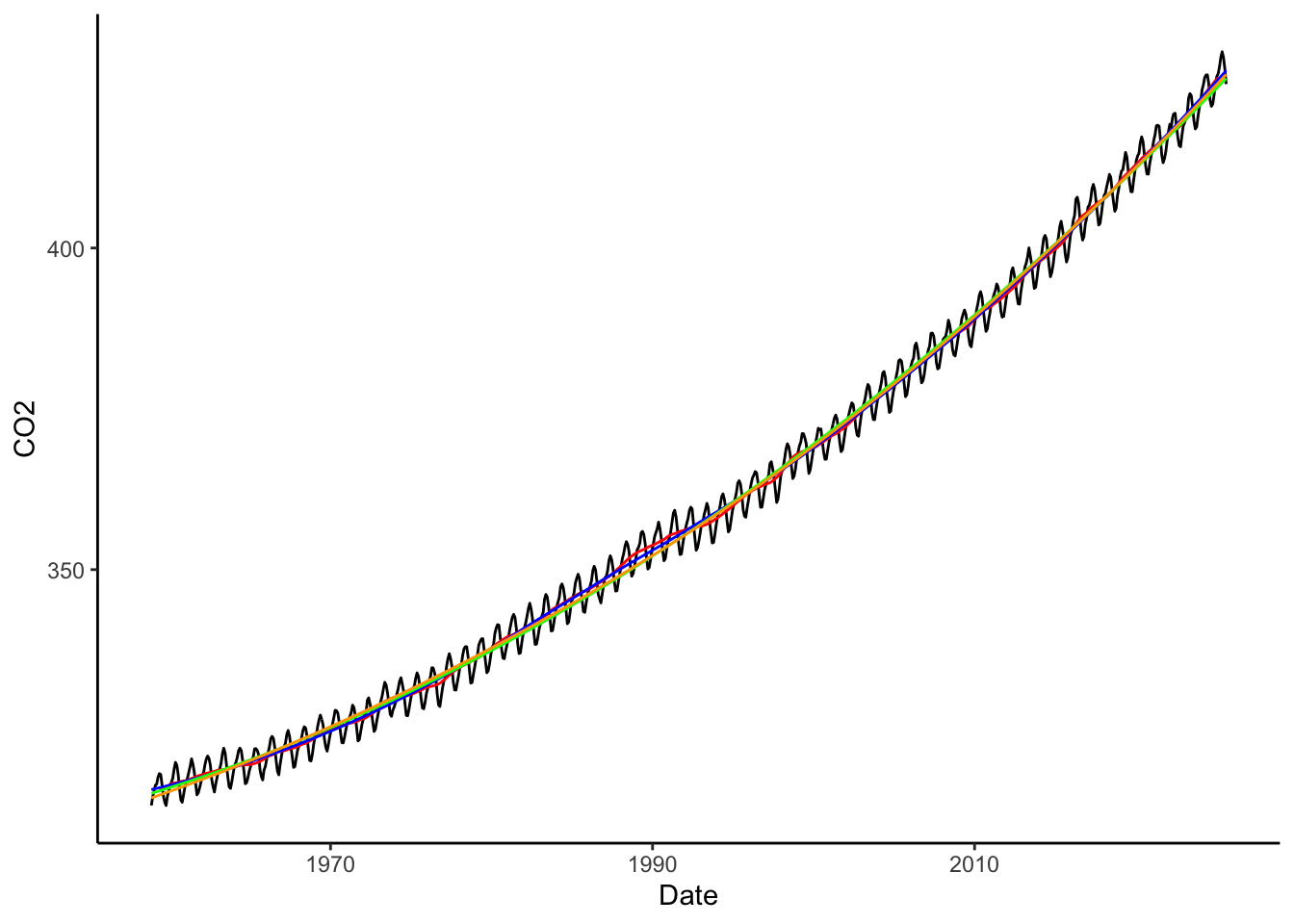
What other ways might we estimate this trend? Think about other classes you’ve taken (Stat 155, Stat 253). Try implementing those approaches to estimating the trend, save the predicted values as co2Trend_1 and co2Trend_2, and compare them to the other two estimated trends by plotting it on top.
# Add new variables, co2Trend_1 and co2Trend_2 to the co2 data set
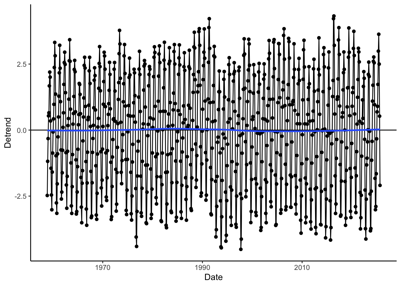
Choose a method (of the four above) to estimate trend that you find works best. Demonstrate its utility on this data set by visualizing the residuals (also known as the detrended data). Make sure the plot includes a horizontal line at 0 and a smooth estimated mean of the residuals across time.
co2 <- co2 %>%mutate(Detrend = CO2 - ??)
Estimating Seasonality
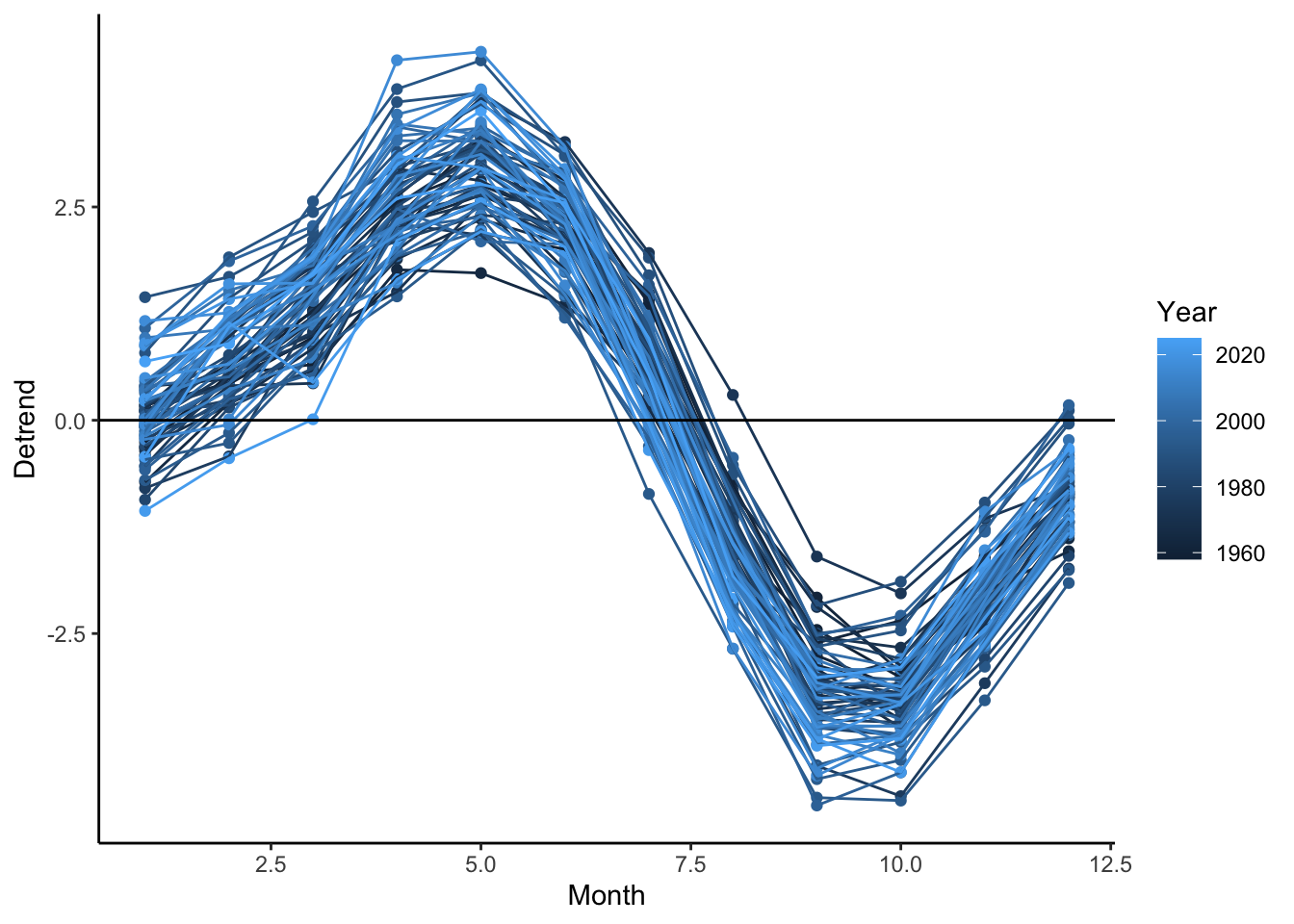
Visualize the seasonality by first removing the estimated trend (the trend you prefer) and plotting those residuals (Detrend) as a function of Month, grouped by Year.
Estimate the seasonality using indicators for Month to estimate the monthly average deviations due to seasonality using linear regression. Plot the estimated average monthly deviations (estimate of the seasonality). Comment on the plot. Does this make sense based on your understanding of the planet and CO2 in the atmosphere?
lm.season <-lm(Detrend ~ ??, data = co2)# Add new variable, Season, as the predictions from lm.season to the co2 data setco2 <- co2 %>%mutate(??) # Plot estimated average monthly deviations
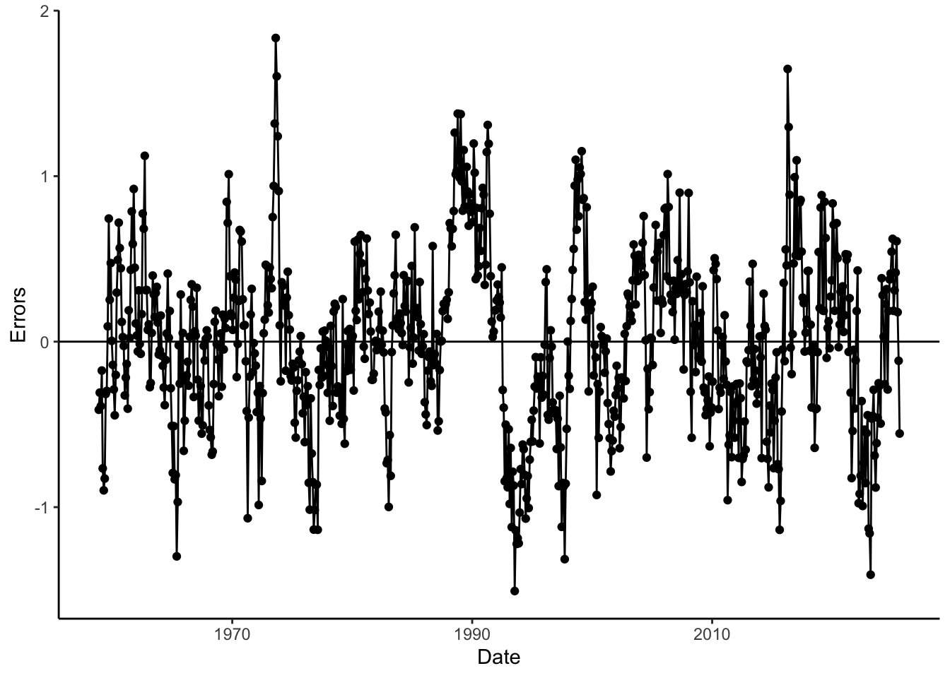
Visualize the leftover residuals after removing the estimated seasonality (Errors). Do the residuals look like independent random noise?
co2 <- co2 %>%mutate(Errors = Detrend - Season)co2 %>%ggplot(aes(x = Date, y = Errors)) +geom_point() +geom_line() +geom_hline(yintercept =0) +theme_classic()
Do you think it is safe to assume the resulting random process is stationary?
Assuming stationarity, estimate the correlation function. Comment and what you notice. What does it mean in the context of the problem? Is it independent random noise?
acf(na.omit(co2$Errors))
We will consider models for these error processes, assuming they are stationary.
CHALLENGE: Let’s say you want to predict the CO2 concentrations in the near future. How could you use what we’ve done so far to do that prediction? How might you adjust the processes we’ve used to make forecasts in the future? Don’t implement, just brainstorm.
Concept: Differencing
If you have time during class, continue working. Otherwise, we’ll come back to this concept in another class activity.
Instead of estimating the trend and seasonality, we could directly remove the trend and seasonality with differencing.
A first-order difference is \(y_t - y_{t-1}\). A first-order seasonal difference with lag 12 is \(y_t - y_{t-12}\).
First-order Differences
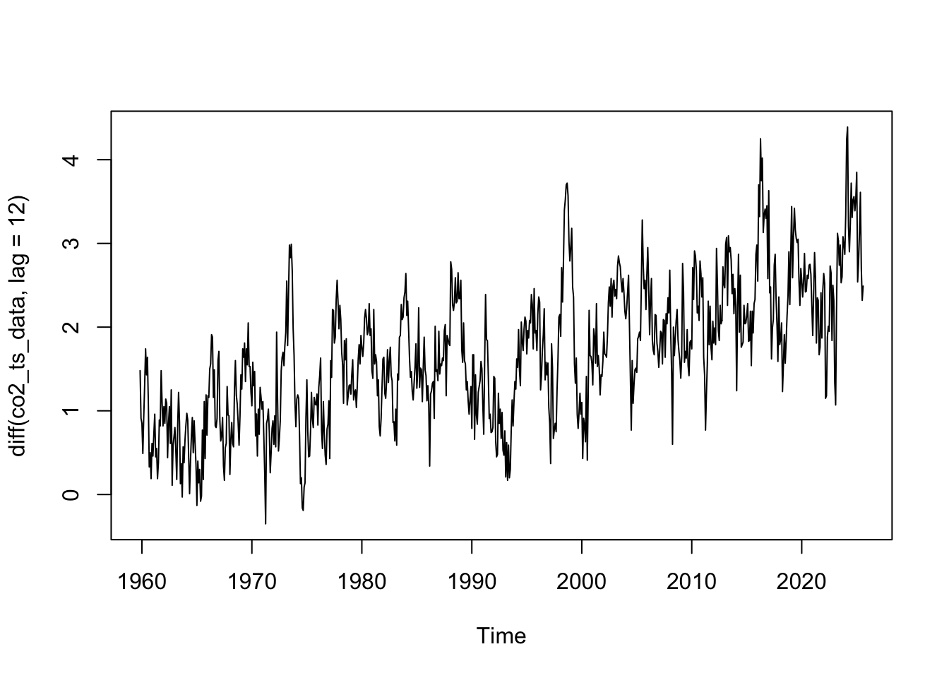
If you take a first-order difference between observations 12 months apart (lag 12), you get this. Describe what is left over.
plot(diff(co2_ts_data,lag =12))
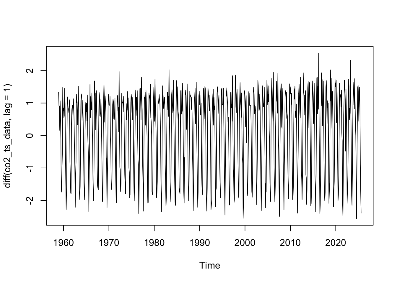
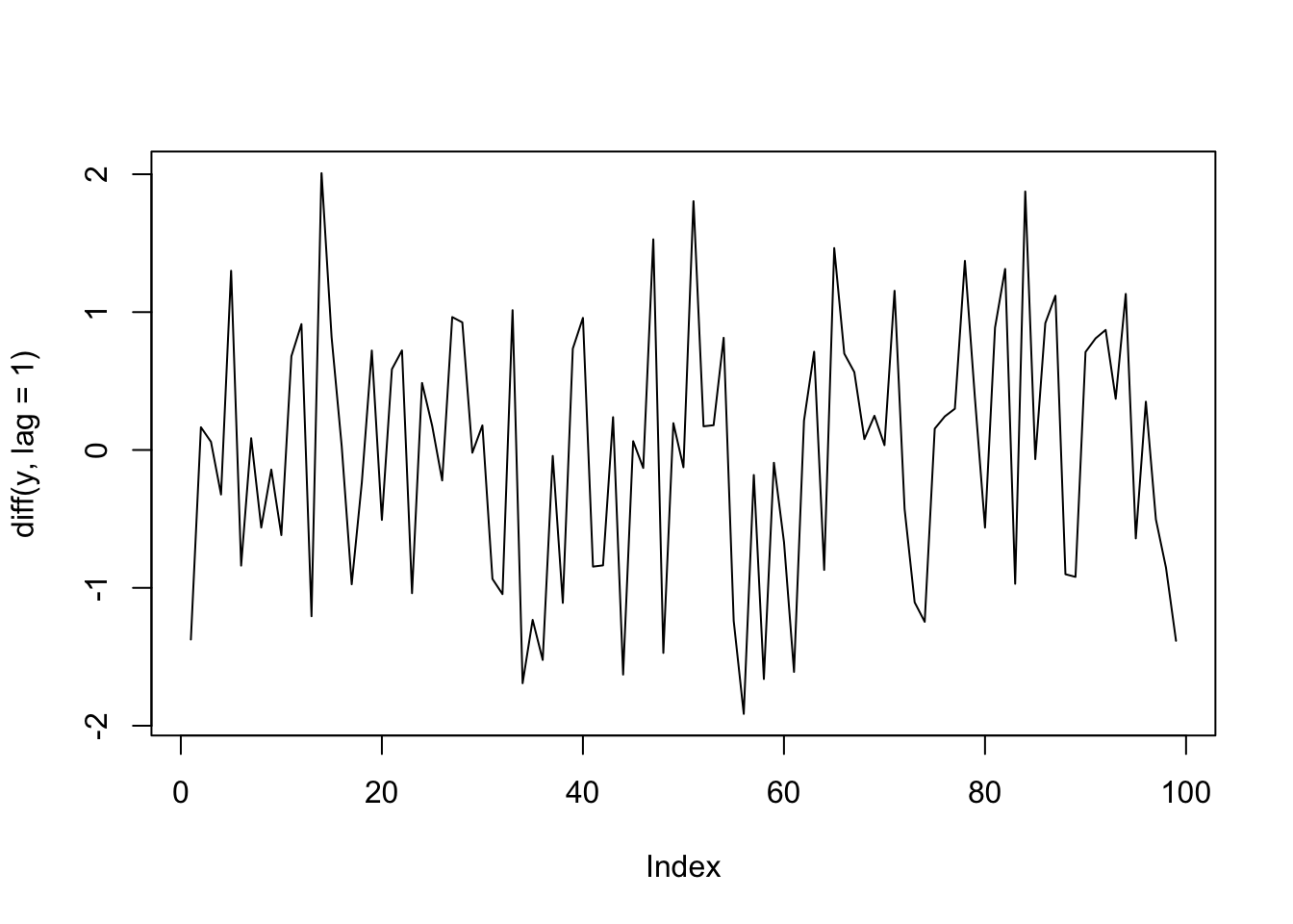
If you take a first-order difference between observations 1 month apart (lag 1), you get this. Describe what is left over.
plot(diff(co2_ts_data,lag =1))
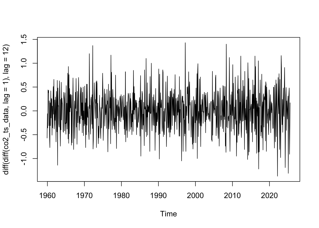
If you take the 1 month differences and then take 12 month differences, we get this. Describe what is left over.
\[(y_t - y_{t-1}) - (y_{t-12} - y_{t-13})\]
plot(diff(diff(co2_ts_data,lag =1),lag =12))
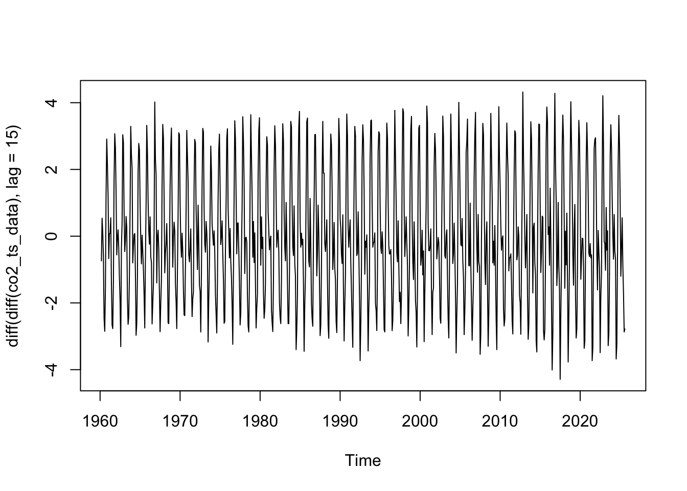
Try a seasonal lag of a different value other than 12, what happens? Describe what is left over.
plot(diff(diff(co2_ts_data),lag = ?))
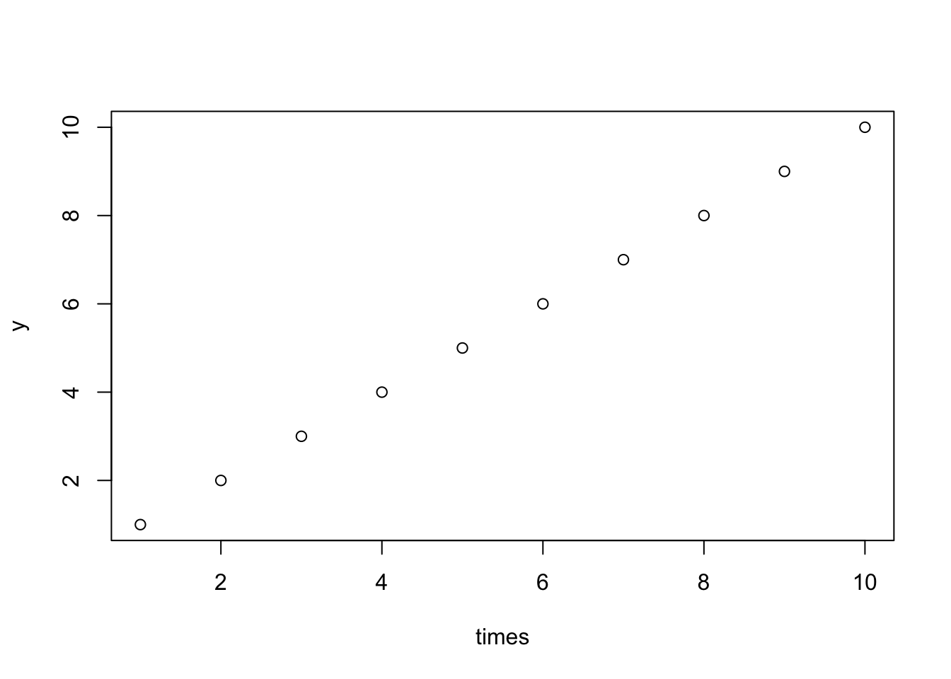
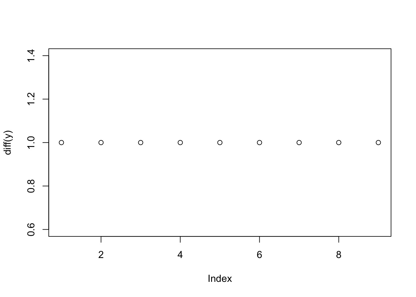
Imagine process with a linear trend line (\(y_t = t\)). What will a first-order difference look like? Prove it to yourself algebraically (and then look at the graph).
\[(y_t - y_{t-1})\]
times =1:10y = timesplot(times, y)plot(diff(y))
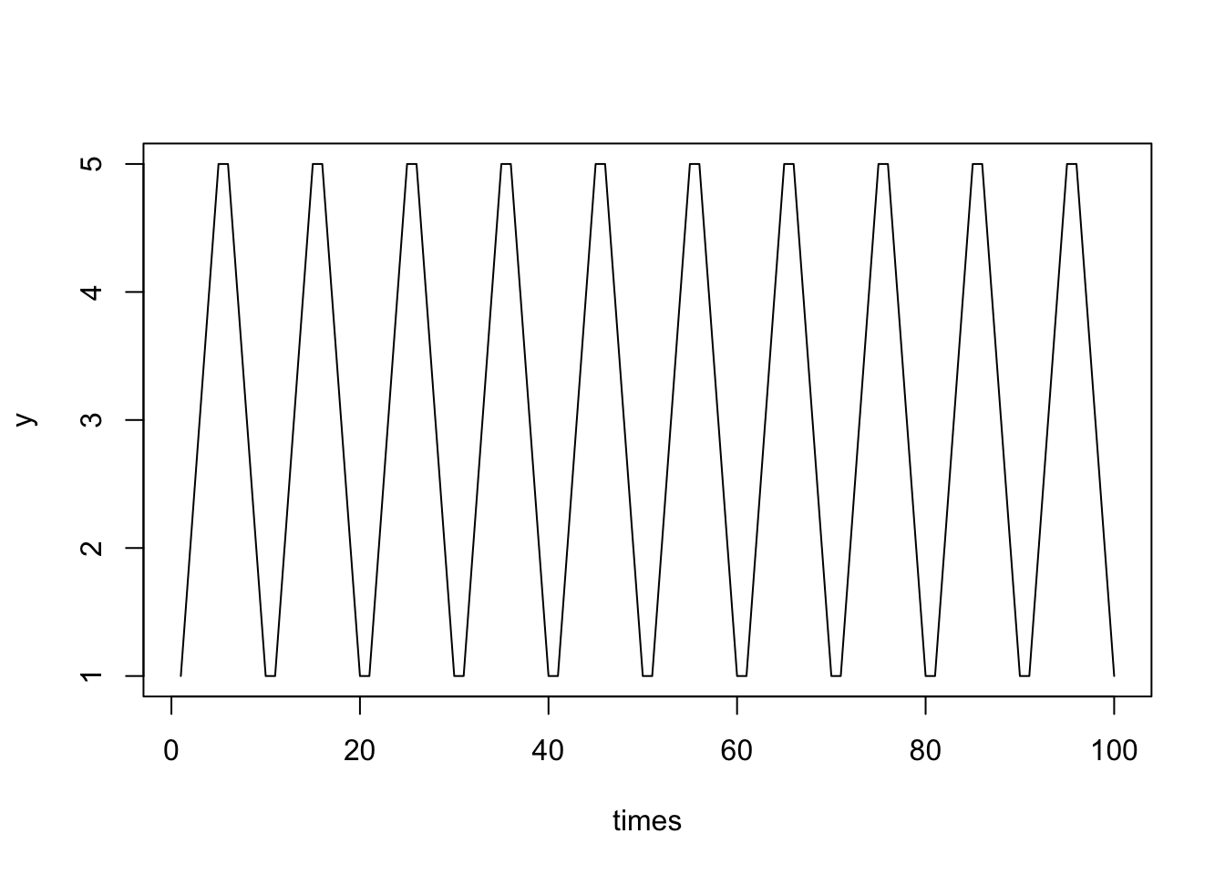
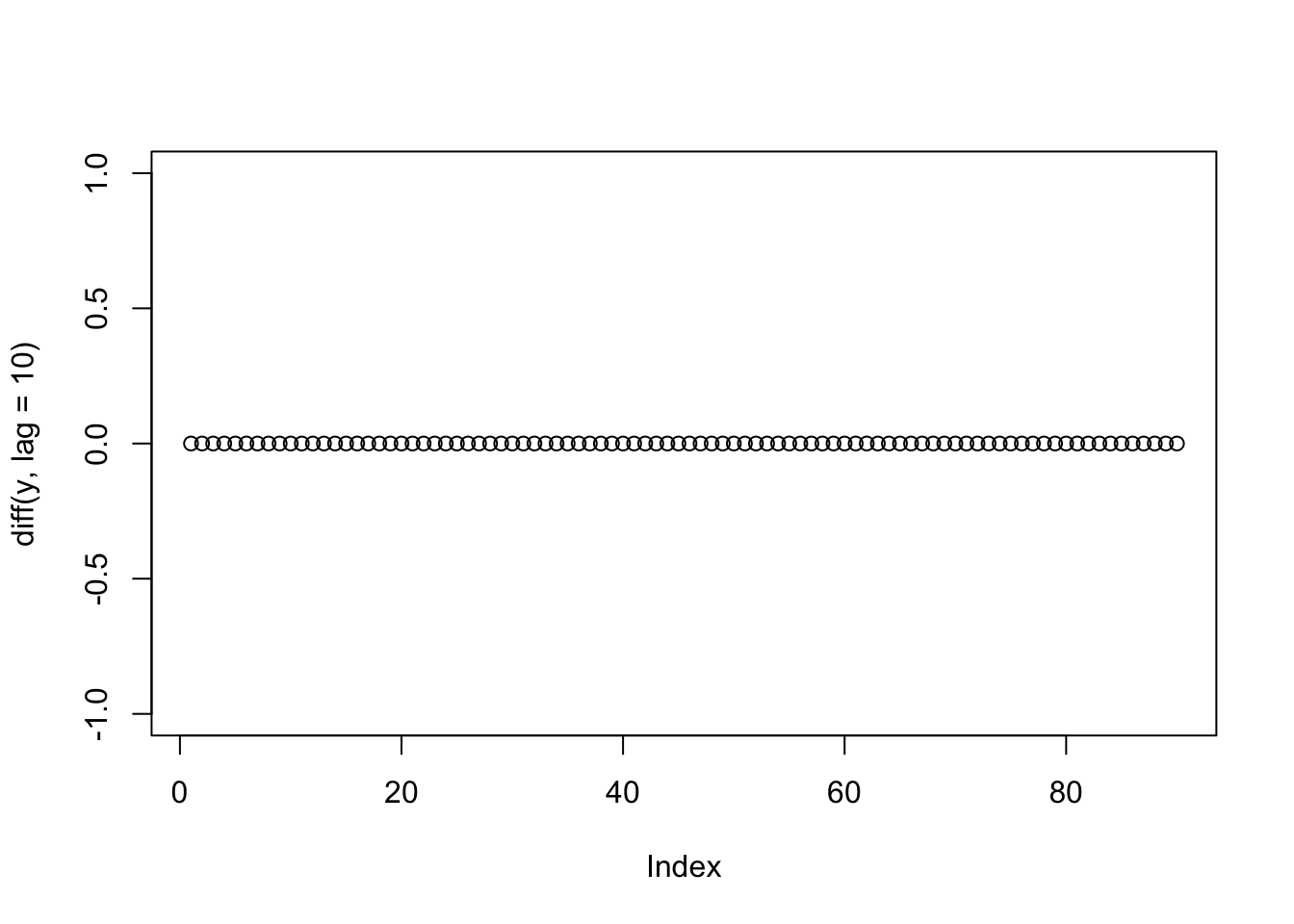
Imagine a process with no trend but a seasonal component where \(y_t = y_{t-k}\). What would a first-order difference of seasonal lag \(k\) do? Prove it to yourself algebraically (and then look at the graph).
\[(y_t - y_{t-k})\]
times =1:100y =rep(c(1:5,5:1),10)plot(times,y,type='l')plot(diff(y, lag=10))
Second-order Differences
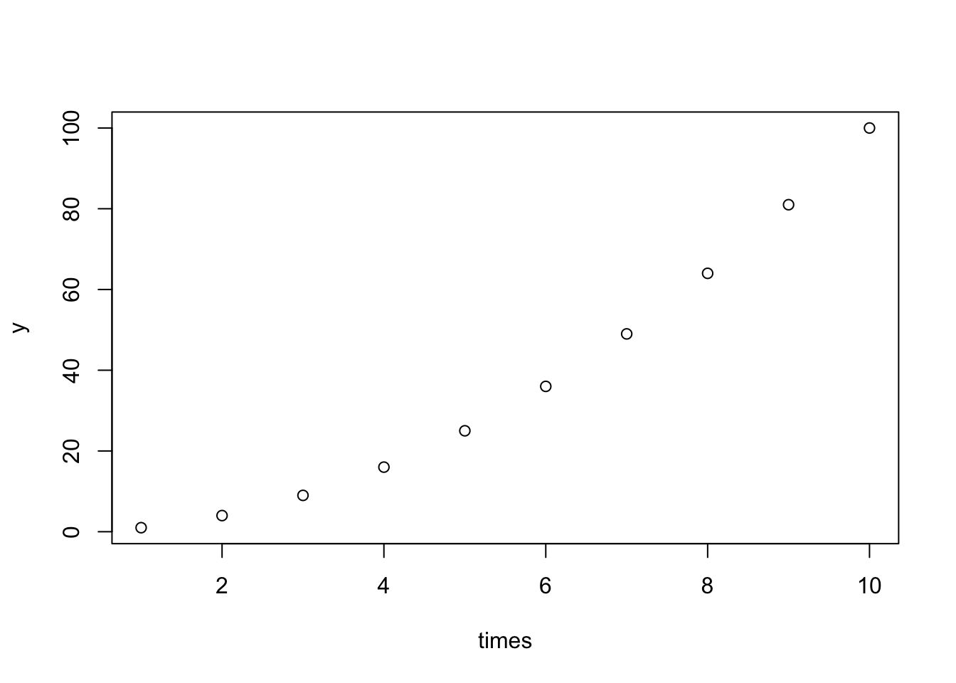
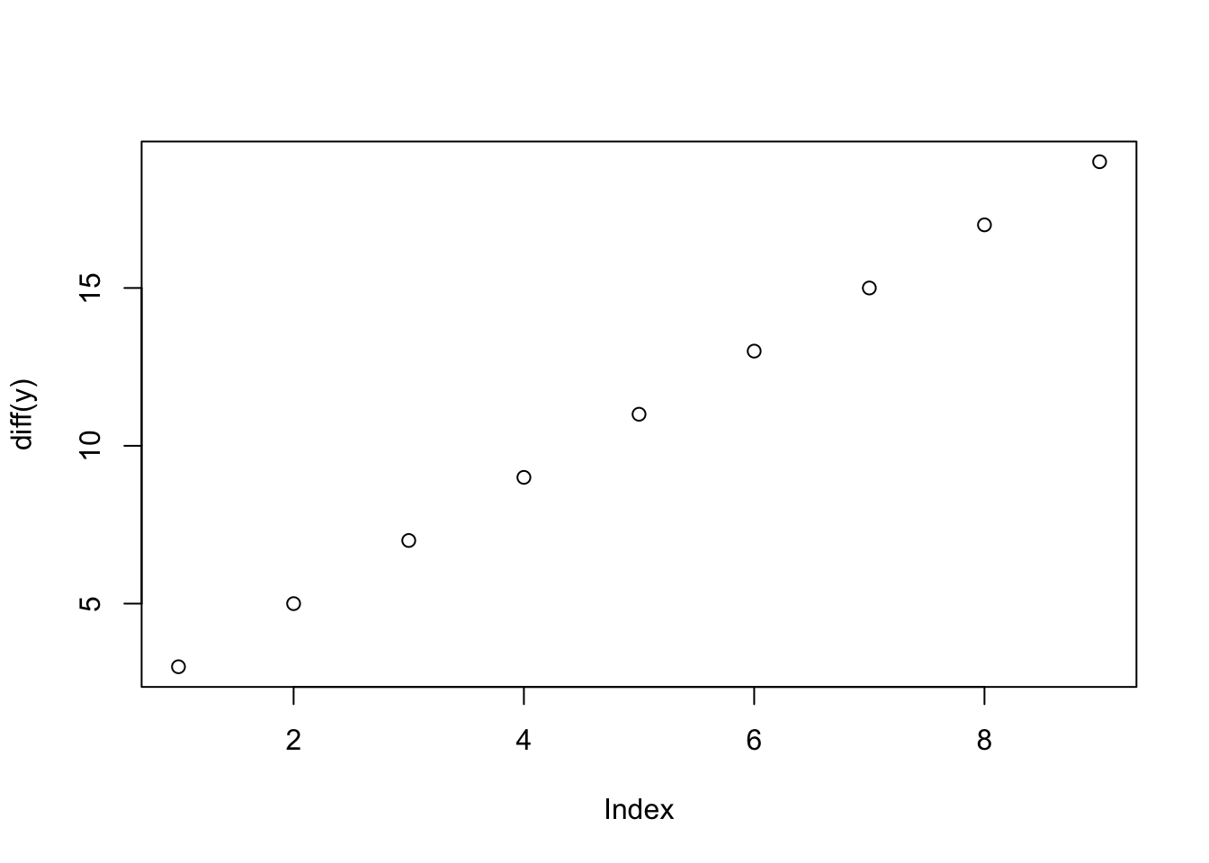
Imagine a random process with quadratic trend (\(y_t = t^2\)). What will a first-order difference look like? Prove it to yourself algebraically (and then look at the graph).
times =1:10y = times^2plot(times,y)plot(diff(y))
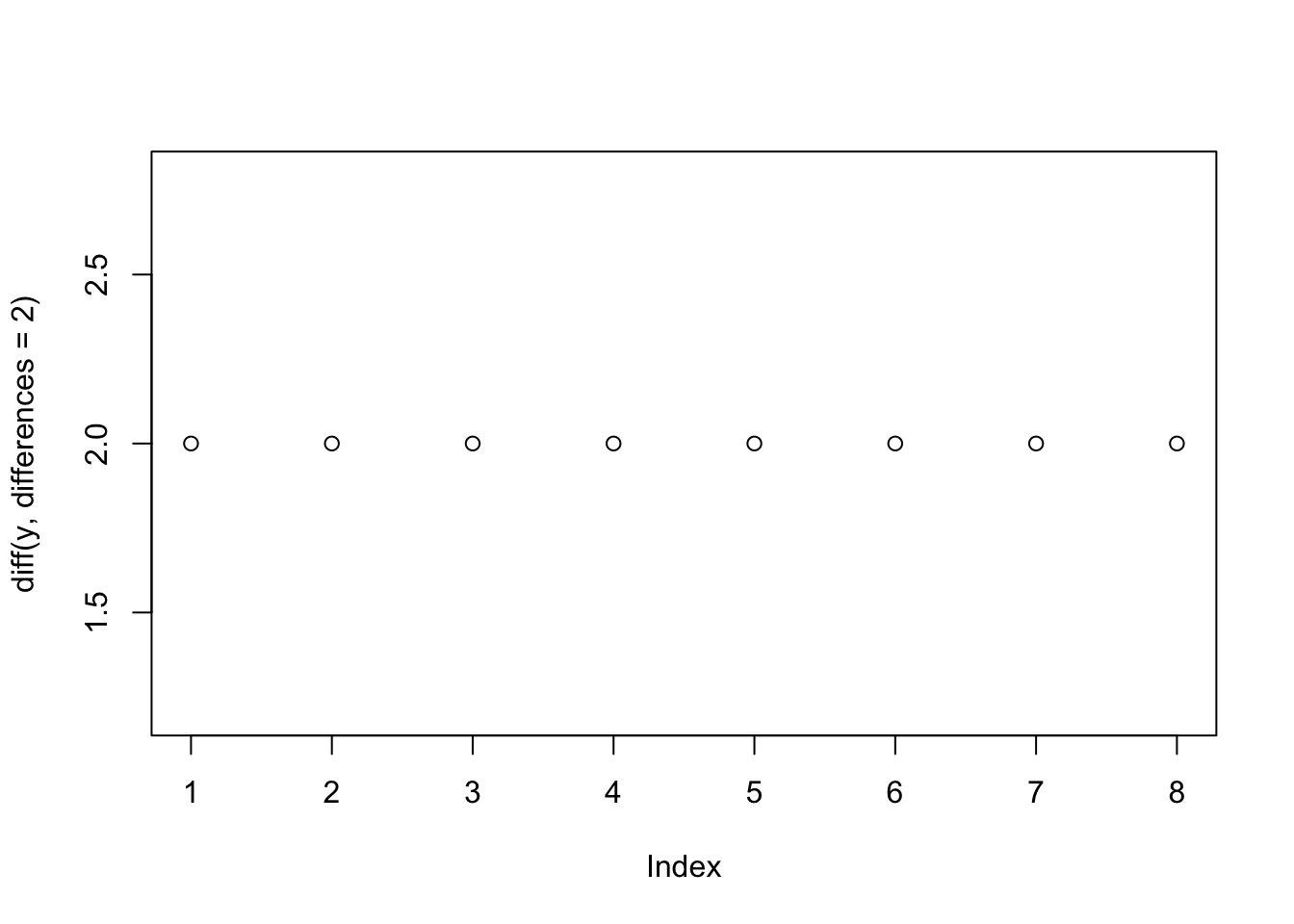
For the process with quadratic trend, what will a second-order difference (difference the difference) look like? Prove it to yourself algebraically (and then look at the graph).
We see that there is a bit of an increase in CO2 concentrations in the spring, that then decrease in the fall.
co2 %>%ggplot(aes(x = Month, y = CO2, group = Year, color = Year)) +geom_point() +geom_line() +theme_classic()
Estimating Trend
.
Solution
co2_ts_data <-ts(co2$CO2, start =c(1958,11), frequency =12) # ts (time series) objects keeps track of timefltr <-c(0.5, rep(1, 11), 0.5)/12#vector of weights for moving average filterco2 <- co2 %>%mutate( co2Trend_MA =as.numeric(stats::filter(co2_ts_data, filter = fltr, method ='convo', sides =2)))co2 %>%ggplot(aes(x = Date, y = CO2)) +geom_line() +geom_line(aes(y = co2Trend_MA), color ='red') +theme_classic()
.
Solution
co2 <- co2 %>%mutate(co2Trend_loess =predict(loess(CO2 ~ Date, data = co2, span =0.5)))co2 %>%ggplot(aes(x = Date, y = CO2)) +geom_line() +geom_line(aes(y = co2Trend_MA), color ='red') +geom_line(aes(y = co2Trend_loess), color ='blue') +theme_classic()
.
Solution
library(splines)co2 <- co2 %>%mutate(co2Trend_1 =predict(lm(CO2 ~poly(Date,2), data = co2))) # quadratic functionco2 <- co2 %>%mutate(co2Trend_2 =predict(lm(CO2 ~bs(Date,knots=c(1990),degree=2), data = co2))) # quadratic splinesco2 %>%ggplot(aes(x = Date, y = CO2)) +geom_line() +geom_line(aes(y = co2Trend_MA), color ='red') +geom_line(aes(y = co2Trend_loess), color ='blue') +geom_line(aes(y = co2Trend_1), color ='green') +geom_line(aes(y = co2Trend_2), color ='orange') +theme_classic()
.
Solution
co2 <- co2 %>%mutate(Detrend = CO2 - co2Trend_loess) # or co2Trend_MA, co2Trend_1, or co2Trend_2co2 %>%ggplot(aes(x = Date, y = Detrend)) +geom_point() +geom_line() +geom_hline(yintercept =0) +geom_smooth(se =FALSE) +theme_classic()
Estimating Seasonality
.
Solution
co2 %>%ggplot(aes(x = Month, y = Detrend, group = Year, color = Year)) +geom_point() +geom_line() +geom_hline(yintercept =0) +theme_classic()
.
Solution
lm.season <-lm(Detrend ~factor(Month), data = co2)co2 <- co2 %>%mutate(Season =predict(lm.season, newdata = co2))co2 %>%ggplot(aes(x = Month, y = Detrend, group = Year)) +geom_point() +geom_line() +geom_line(aes(y = Season), color ='purple', size =2) +geom_hline(yintercept =0) +theme_classic()
.
Solution
No, they do not look independent.
co2 <- co2 %>%mutate(Errors = Detrend - Season)co2 %>%ggplot(aes(x = Date, y = Errors)) +geom_point() +geom_line() +geom_hline(yintercept =0) +theme_classic()
.
Solution
Maybe. The mean looks on average to be 0, the variance is relatively constant, and it is hard to tell about the covariance just from a plot of the data.
.
Solution
There is a decay in the autocorrelation to zero such that by 15 months apart, there is virtually 0 correlation between observations. No, it is not independent random noise.
acf(na.omit(co2$Errors))
Solution
We could take our trend and seasonality and try to extend that into the future (which is easier with parametric methods) and then incorporate the autocorrelation of errors in some how.
Concept: Differencing
First-order Differences
.
Solution
After a first-order difference 12 months apart, we have removed the seasonality of the data but we still have an upward trend!
plot(diff(co2_ts_data,lag =12))
.
Solution
After a first-order difference 1 months apart, we have removed the trend but we still have seasonality in the data!
plot(diff(co2_ts_data,lag =1))
.
Solution
We get data that looks like it no longer has a trend or seasonality.
plot(diff(diff(co2_ts_data,lag =1),lag =12))
Solution
If we use a lag other than the period of the cycle (12 in this data), we still have cyclic behavior over time.
plot(diff(diff(co2_ts_data),lag =15))
.
Solution
A first-order difference removes linear trends.
times =1:10y = timesplot(times, y)
plot(diff(y))
.
Solution
A first-order seasonal difference removes seasonality.
times =1:100y =rep(c(1:5,5:1),10)plot(times,y,type='l')
plot(diff(y, lag=10))
Second-order Differences
.
Solution
A first-order difference on a quadratic curve leaves a linear trend.
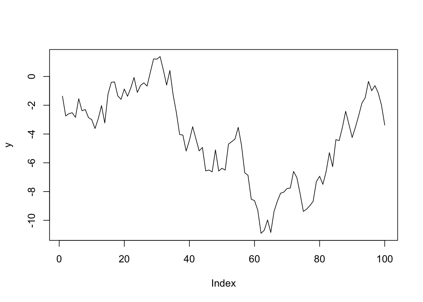
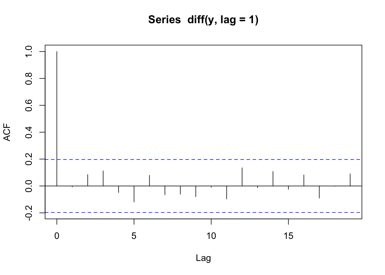
A first-order difference would leave \(\epsilon_t\), the independent random error.
e =rnorm(100)y =cumsum(e)plot(y,type='l')
plot(diff(y, lag=1),type='l')
acf(diff(y, lag=1))
Wrap-Up
Finishing the Activity
If you didn’t finish the activity, no problem! Be sure to complete the activity outside of class, review the solutions in the online manual, and ask any questions on Slack or in office hours.
Re-organize and review your notes to help deepen your understanding, solidify your learning, and make homework go more smoothly!
After Class
Before the next class, please do the following:
Take a look at the Schedule page to see how to prepare for the next class.