# Linear Mixed Effects Model
# Subject-specific parameter specified in ( ___ | id)

lme4::lmer(Y ~ X1 + X2 + (1 | id), data = data, REML = TRUE) %>%
  summary() # prints out estimates, model SE, t-values


lme4::lmer(Y ~ X1 + X2 + (X1 | id), data = data , REML = TRUE) %>%
summary() # prints out estimates, model SE, t-values12 Mixed Effects
Settling In
Highlights from Day 11
Generalized Estimating Equations (GEE)
Definition: Generalized Estimating Equations is an approach to estimate the parameters of a Marginal Model version of a GLM with correlation among repeated measures of longitudinal data.
. . .
GEE is a semi-parametric approach that estimates coefficients by solving the following estimating equations:
\[0 = \sum_{i=1}^n \frac{\partial \boldsymbol\mu_i}{\partial \boldsymbol\beta }\mathbf{V}_i^{-1}(\mathbf{Y}_i - \boldsymbol\mu_i(\boldsymbol \beta)) \]
where \(\mathbf{V}_i\) is a covariance matrix based on a working correlation structure and \(\boldsymbol\mu_i(\boldsymbol\beta)\) is based on a link function and a linear combination of X variables, \(\mu_{ij}(\boldsymbol\beta) = g^{-1}(\mathbf{x}_{ij}^T\boldsymbol\beta)\), and
\[\mathbf{V}_i = \mathbf{A}_i^{1/2} Cor(\mathbf{Y}_i) \mathbf{A}_i^{1/2}\]
where \(\mathbf{A}_i\) is a diagonal matrix with \(Var(Y_{ij} | X_{ij}) = \phi v(\mu_{ij})\) along the diagonal.
. . .
If an observation is missing completely at random (MCAR), the estimates are still valid.
If an observation is not missing completely at random, one could incorporate inverse-probability weights that account for drop out / missing values if the missingness is associated with other variables that are observed (called MAR).
Learning Goals
- Explain and illustrate a random intercept model and connect to compound symmetry model
- Explain how random intercepts and slopes model correlation
- Fit mixed effects models to real data and interpret the output
Mixed Effects Models
Definitions
Generalized Linear Mixed Effects is a longitudinal model that incorporates correlation within subjects.
. . .
Mixed Effects Model is similar to a GLM (Distribution, Link function, Systematic component), except we incorporate subject-specific parameters in the Systematic Component of the mean model,
\[g(E[\mathbf{Y}_{i} | \mathbf{X}_{i}, \mathbf{Z}_{i},\mathbf{b}_i ]) = \mathbf{X}_{i}\boldsymbol\beta + \mathbf{Z}_i\mathbf{b}_i \]
. . .
The Mixed Effects Model involves fixed effects and random effects.
- It models the mean with population-level parameters \(\boldsymbol\beta\), similar to GLM (fixed effects).
- These are the parameters you are primarily interested in, that are common within the population (e.g., the association with a new drug, the association with age).
- It models “within-subject” correlation with subject-specific parameters, \(\mathbf{b}_i\), that are treated as random variables (random effects).
- Random effects represent the variability attributable to the groups or individuals themselves (e.g., differences in average response between individuals, or differences in slopes of change over time between individuals).
- You’re typically not interested in the specific effect of each individual group, but rather in the overall variance attributable to that grouping factor.
- Note: If you have multiple levels of correlation (time and space), you can model these different sources of (co)-variation.
Model Specification
For now, we’ll focus on quantitative, continuous outcomes.
We can write a linear mixed effects model in terms of our (quantitative) outcome vector,
\[\mathbf{Y}_{i} = \mathbf{X}_{i}\boldsymbol\beta + \mathbf{Z}_i\mathbf{b}_i + \boldsymbol\epsilon_i,\quad\quad \boldsymbol\epsilon_i\sim N(0,\boldsymbol\Sigma), \mathbf{b}_i\sim N(0,\mathbf{G}), \boldsymbol\epsilon_i \perp \mathbf{b}_i\]
\[= \text{Fixed effects} + \text{Random effects} + \text{Error}\]
where
- \(\mathbf{X}_i\) is the model matrix for the fixed effects,
- \(\mathbf{Z}_i\) is the model matrix for the random effects (a subset of columns of \(\mathbf{X}_i\)),
- \(\boldsymbol\epsilon_i\sim N(0,\boldsymbol\Sigma)\),
- \(\mathbf{b}_i\sim N(0,\mathbf{G})\), and
- \(\mathbf{b}_i\) and \(\boldsymbol\epsilon_i\) are independent of each other.
. . .
Thus,
\[\mathbf{Y}_{i}\sim N(\mathbf{X}_{i}\boldsymbol\beta,\mathbf{Z}_i\mathbf{G}\mathbf{Z}_i^T + \boldsymbol\Sigma)\quad\quad \boldsymbol\epsilon_i\sim N(0,\boldsymbol\Sigma), \mathbf{b}_i\sim N(0,\mathbf{G}), \boldsymbol\epsilon_i \perp \mathbf{b}_i \]
Typically, we assume \(\boldsymbol\Sigma = \sigma^2_{\epsilon} I\).
Properties
If the full model is correct \[\mathbf{Y}_i = \mathbf{X}_i\boldsymbol\beta + \mathbf{Z}_i\mathbf{b}_i + \boldsymbol\epsilon_i\quad\quad \boldsymbol\epsilon_i\sim N(0,\boldsymbol\Sigma), \mathbf{b}_i\sim N(0,\mathbf{G}), \boldsymbol\epsilon_i \perp \mathbf{b}_i,\]
. . .
then the marginal expected value of the outcome is
\[ E(\mathbf{Y}_i| \mathbf{X}_{i}, \mathbf{Z}_{i}) = E(\mathbf{X}_i\boldsymbol\beta + \mathbf{Z}_i\mathbf{b}_i + \boldsymbol\epsilon_i | \mathbf{X}_{i}, \mathbf{Z}_{i})\] \[ = E(\mathbf{X}_i\boldsymbol\beta | \mathbf{X}_{i}, \mathbf{Z}_{i}) +E(\mathbf{Z}_i\mathbf{b}_i | \mathbf{X}_{i}, \mathbf{Z}_{i}) + E(\boldsymbol\epsilon_i| \mathbf{X}_{i}, \mathbf{Z}_{i})\] \[ = E(\mathbf{X}_i\boldsymbol\beta | \mathbf{X}_{i}, \mathbf{Z}_{i}) = \mathbf{X}_i\boldsymbol\beta \]
. . .
the conditional expected value of the outcome is
\[ E(\mathbf{Y}_i| \mathbf{X}_{i}, \mathbf{Z}_{i}, \mathbf{b}_{i}) = E(\mathbf{X}_i\boldsymbol\beta + \mathbf{Z}_ib_i + \boldsymbol\epsilon_i | \mathbf{X}_{i}, \mathbf{Z}_{i}, \mathbf{b}_{i})\] \[ = E(\mathbf{X}_i\boldsymbol\beta | \mathbf{X}_{i}, \mathbf{Z}_{i}, \mathbf{b}_{i}) +E(\mathbf{Z}_i\mathbf{b}_i | \mathbf{X}_{i}, \mathbf{Z}_{i}, \mathbf{b}_{i}) + E(\boldsymbol\epsilon_i| \mathbf{X}_{i}, \mathbf{Z}_{i}, \mathbf{b}_{i})\] \[ = \mathbf{X}_i\boldsymbol\beta + \mathbf{Z}_i\mathbf{b}_i\]
. . .
The covariance of the outcome is
\[ Cov(\mathbf{Y}_i) = Cov(\mathbf{X}_i\boldsymbol\beta + \mathbf{Z}_ib_i + \boldsymbol\epsilon_i)\] \[ = Cov(\mathbf{Z}_i\mathbf{b}_i) + Cov(\boldsymbol\epsilon_i)\] \[ = \mathbf{Z}_iCov(\mathbf{b}_i)\mathbf{Z}_i^T + Cov(\boldsymbol\epsilon_i)\] \[ = \mathbf{Z}_i\mathbf{G}\mathbf{Z}_i^T + \boldsymbol\Sigma\]
Implementation
To estimate a mixed effects model, we can use the lme4 package in R.
We can use the lmer function for linear mixed effects models and the glmer function for generalized linear mixed effects models (e.g., logistic regression).
- Estimation could be done with Restricted Maximum Likelihood (REML) or Maximum Likelihood (ML). REML is often preferred for mixed effects models because it accounts for the estimation of the random effects variance separately from the fixed effects.
. . .
The basic syntax is:
# Logistic Linear Mixed Effects Model
lme4::glmer(Y ~ X1 + X2 + (1 | id), family = binomial, data = data, REML = TRUE) %>%
  summary() # prints out estimates, model SE, t-values
Warm Up
Random Intercept Model
Using the notation, define \(\mathbf{Z}_i\), \(\mathbf{b}_i\), and \(\mathbf{G}\) for a random intercept model.
If we use a random intercept model and we assume \(\boldsymbol\Sigma = \sigma^2_{\epsilon} I\), describe the structure of \(Cov(Y_i) = \mathbf{Z}_i\mathbf{G}\mathbf{Z}_i^T + \boldsymbol\Sigma\).
Random Slope Model
Using the notation, define \(\mathbf{Z}_i\), \(\mathbf{b}_i\), and \(\mathbf{G}\) for a random slope model.
If we use a random slope model and we assume \(\boldsymbol\Sigma = \sigma^2_{\epsilon} I\), describe the structure of \(Cov(Y_i) = \mathbf{Z}_i\mathbf{G}\mathbf{Z}_i^T + \boldsymbol\Sigma\).
Model Selection
When selecting models, we must consider:
- Model Type
- Mean Model
- Covariance Model
Choices
- Model Type: Pros and Cons (Mixed Effects v. GEE)
- Desired Interpretation
- Mean Model: Which X’s
- Research Question
- Research Goals (Causal Inference v. Approximate a relationship)
- Covariance Model: Structure or Random Effects
- Data Context
- Resulting Covariance
- Goodness of Fit to Data
Hypothesis Testing Coefficients
In order to test fixed effects, use ML and not REML, then we can test whether \(\beta_k=0\) for some \(k\).
. . .
In mixed effects models, the estimated covariance matrix for \(\hat{\boldsymbol\beta}\) is \[\widehat{Cov}(\hat{\boldsymbol\beta}) = \left\{ \sum^n_{i=1} \mathbf{X}_i^T\hat{\mathbf{V}}_i\mathbf{X}_i \right\}^{-1}\]
The standard error for \(\hat{\beta}_k\) is the square rooted values of the diagonal of this matrix corresponding to \(\hat{\beta}_k\). This is what is reported in the summary output.
. . .
To test the hypothesis \(H_0: \beta_k=0\) vs. \(H_A: \beta_k\not=0\), we can calculate a t-statistic,
\[t = \frac{\hat{\beta}_k}{SE(\hat{\beta}_k)} \]
With mixed effects models, there is debate about what the appropriate distribution of this statistic is, which is why p-values are often not reported in the output. However, if you have an estimate that is large relative to the standard error (greater than 2 SE’s away), that is a good indication that it is significantly different from zero.
summary(mod1)

# Manual Code to get t-values

fixef(mod1)/sqrt(diag(vcov(mod1)))
Hypothesis Testing Groups of Coefficients
To compare two models (same random effects and same covariance models, but set some \(\beta\)’s to 0), we could use a likelihood ratio test. Suppose we have two models with the same random effects and covariance models,
- Full model: \(M_f\) has \(p+1\) columns in \(\mathbf{X}_i\) and thus \(p+1\) fixed effects \(\beta_0,...,\beta_{p}\).
- Nested model: \(M_n\) has \(k+1\) columns such that \(k < p\) and \(p-k\) fixed effects \(\beta_l = 0\).
. . .
If we are using maximum likelihood estimation (not REML), it makes sense to compare the likelihood of the two models.
\(H_0:\) nested model is true, \(H_A:\) full model is true
. . .
If we take the ratio of the likelihoods from the nested model and full model and plug in the maximum likelihood estimators, then we have another statistic.
\[D = -2\log\left(\frac{L_n(\hat{\boldsymbol\beta},\hat{\mathbf{V}})}{L_f(\hat{\boldsymbol\beta},\hat{\mathbf{V}})}\right) = -2 \log(L_n(\hat{\boldsymbol\beta},\hat{\mathbf{V}})) + 2\log(L_f(\hat{\boldsymbol\beta},\hat{\mathbf{V}}))\]
The sampling distribution of this statistic is approximately chi-squared with degrees of freedom equal to the difference in the number of parameters between the two models.
anova(mod1, mod2) # mod2 is a nested model of mod1Goodness of Fit: Information Criteria
To choose between two models, we can use the Bayesian Information Criterion (BIC). BIC is a model selection criterion that penalizes the likelihood of the model by the number of parameters and the sample size. Choose a model with a lower BIC (higher likelihood, fewer parameters).
\[BIC= -2\log(\hat{L}(\hat{\boldsymbol\beta},\hat{\mathbf{V}})) + k\log(n)\]
where \(\hat{L}(\hat{\boldsymbol\beta},\hat{\mathbf{V}})\) is the likelihood of the model with estimated parameters \(\hat{\boldsymbol\beta}\) and covariance matrix \(\hat{\mathbf{V}}\), \(k\) is the number of parameters in the model, and \(n\) is the number of observations.
- To choose between two models with different random effects, only compare models with the same fixed effects.
Note: In order to use BIC to choose between mixed effects models, you must use maximum likelihood (ML) estimation instead of REML.
Model Diagnostics
For any linear model, we should check to see if the residuals have no pattern.
data %>%
  mutate(Pred = predict(mod)) %>%
  mutate(Resid = resid(mod)) %>%
  ggplot(aes(x = Pred, y = Resid)) +
  geom_point(alpha = .2) +
  geom_hline(yintercept = 0) +
  geom_smooth(se = FALSE) +
  theme_classic()
For a mixed effects model, you are assuming the random effects distribution is Normal.
- You should check on the distribution of the predicted random effects to see if they are approximately Normal.
A <- ranef(mod)
qqnorm(A)
qqline(A)
Small Group Activity
Download a template Qmd file to start from here.
Exercises
source('Cleaning.R') #Open Cleaning.R for information about variables.
head(activeLong)- We are going to consider modeling
Memoryas a function ofYearsand treatment groupINTGRPwith a mixed effects model. Let’s start by using a random intercept model. Describe the assumptions made by the code below. Consider the assumptions about the model for the mean (fixed effects) and the assumptions about the random effects.
activeLong <- activeLong %>% mutate(INTGRP = relevel(INTGRP, ref='Control'))

library(lme4)
library(tidyr)
mod1 <- activeLong %>% drop_na(Memory, Years, INTGRP) %>%
  lmer(Memory ~ Years*I(Years > 3)*INTGRP + (1|AID), data = ., REML = FALSE)

mod1 %>% summary()- Compare the estimated coefficients between the random intercept model and the GEE with an exchangeable working correlation structure. Describe what you observe and explain why it is so.
mod2 <- activeLong %>% drop_na(Memory,Years,INTGRP) %>%
  geeM::geem(Memory ~ Years*I(Years > 3)*INTGRP, data = ., id = AID, corstr = 'exchangeable')

tibble(MixedBeta = fixef(mod1) %>% round(2), GEEBeta =  mod2$beta %>% round(2)) %>%
mutate(Diff = MixedBeta - GEEBeta) - Compare the estimated standard errors between the random intercept model and the GEE with an exchangeable working correlation structure (GEE have naive/model-based and robust SE’s). Describe what you observe and explain why it might be so.
tibble(MixedSE = vcov(mod1) %>% diag() %>% sqrt() %>% round(2),
       GEENaivSE =  mod2$naiv.var %>% diag() %>% sqrt() %>% round(2),
       GEERobustSE =  mod2$var %>% diag() %>% sqrt() %>% round(2)) %>%
mutate(Diff = MixedSE- GEENaivSE, Diff2 = MixedSE- GEERobustSE) - Now, to get a sense of the random intercept model, let’s look at a visualizations of the predictions. First, the predictions are based on the fixed effects and the random effects. The second includes the predictions from the fixed effects. Comment on what you observe and how it relates to the assumptions you made within the model.
activeLong %>% drop_na(Memory, Years, INTGRP) %>%
  mutate(Pred = predict(mod1)) %>%
  ggplot(aes(x = Years, y = Pred, color = INTGRP, group = AID)) +
  geom_line(alpha = .2) +
  labs(color = 'Treatment Group', y = 'Predicted Outcomes (including random effects)') + theme_classic()

activeLong %>% drop_na(Memory, Years, INTGRP) %>%
  mutate(Pred = predict(mod1, re.form = NA)) %>%
  distinct(Years,INTGRP,Pred) %>%
  ggplot(aes(x = Years, y = Pred, color = INTGRP)) +
  geom_line() +
  labs(color = 'Treatment Group', y = 'Predicted Outcomes (only fixed effects)') + theme_classic()
Looking back on the mixed effects model you fit, what do you conclude about the influence of Memory Training (as compared to Control Group) on Memory Score over time.
Compare these three models. Discuss whether your should favor the larger model or the nested models. In other words, do we have evidence that the treatment group is related to how Memory changes over time on average?
For mixed effects models, here is some example code that allows us to test whether the interactions between INTGRP and Years are needed (remove them in mod4, which is equivalent to setting them all to 0; remove the interactions for Speed and Reasoning training in mod4 but keep the interaction with Memory).
mod3 <- activeLong %>% drop_na(Memory,Years,INTGRP) %>%
  lmer(Memory ~ Years*I(Years > 3)*I(INTGRP == 'Memory Training') + (1|AID), data = ., REML = FALSE)

mod4 <- activeLong %>% drop_na(Memory,Years,INTGRP) %>%
  lmer(Memory ~ Years*I(Years > 3) + INTGRP + (1|AID), data = ., REML = FALSE)

anova(mod1, mod4)
anova(mod1, mod3)- Discuss which set of fixed effects seems the best using the Bayesian Information Criteria.
BIC(mod1)
BIC(mod3)
BIC(mod4)- Discuss which set of random effects seems the best using the Bayesian Information Criteria.
mod5 <- activeLong %>% drop_na(Memory,Years,INTGRP) %>%
  lmer(Memory ~ Years*I(Years > 3)*I(INTGRP == 'Memory Training') + (Years|AID), data = ., REML = FALSE)

BIC(mod3)
BIC(mod5)- Lastly, all of these model selection tools are only valid if the entire model is correct (right mean model, right random effects, distributional assumptions about random effects and errors). Check diagnostics and discuss the limitations of your model with this context in mind.
Note about Fixed Effects v. Random Effects
Economics Prefers Fixed Effects
In Econometrics, faculty will suggest including subject-specific parameters as fixed effects rather than random effects.
- Estimating the subject-specific intercepts as parameters (instead of random variables)
For example, if you have longitudinal data for each country over time, you might include country id or name as a fixed effect.
lm(GDP ~ Population + Inflation + Country, data = data). . .
Economics Main Goals
- Omitted Variable Bias and Endogeneity (unobserved variables that are correlated to observed variables)
- Causal Inference
Why Economics use Fixed Effects Models
- \(\mathbf{b}_i\) and \(\boldsymbol\epsilon_i\) might not be independent
- Fixed Effects results in consistency in estimates of interest even if there is omitted variable bias
Solutions
Mixed Effects
Random Intercept Model
Solution
\[\mathbf{Z}_i = \left[\begin{array}{c}1\\1\\ \vdots\\ 1\\1 \end{array}\right]\]
\[\mathbf{b}_i = \left[\begin{array}{c}b_{i0} \end{array}\right]\]
\[\mathbf{G} = \left[\begin{array}{c}\sigma_{0}^2 \end{array}\right]\]
If we use a random intercept model and we assume \(\boldsymbol\Sigma = \sigma^2_{\epsilon} I\), describe the structure of \(Cov(Y_i) = \mathbf{Z}_i\mathbf{G}\mathbf{Z}_i^T + \boldsymbol\Sigma\).
\[Cov(Y_i) = \mathbf{Z}_i\mathbf{G}\mathbf{Z}_i^T + \boldsymbol\Sigma\] \[= \left[\begin{array}{c}1\\1\\ \vdots\\ 1\\1 \end{array}\right]\left[\begin{array}{c}\sigma_{0}^2 \end{array}\right]\left[\begin{array}{ccccc}1&1& \cdots& 1&1 \end{array}\right] + \sigma^2_{\epsilon} I\]
\[= \sigma_{0}^2\left[\begin{array}{ccccc}1&1& \cdots& 1&1 \\1&1& \cdots& 1&1 \\ 1&1&\ddots&1&1\\ 1&1& \cdots& 1&1 \\1&1& \cdots& 1&1 \end{array}\right] + \sigma^2_{\epsilon} I\] Compound Symmetric Structure!
Random Slope Model
Solution
\[\mathbf{Z}_i = \left[\begin{array}{cc}1&x_{i1}\\1&x_{i2}\\ \vdots&\vdots\\ 1&x_{im_i} \end{array}\right]\]
\[\mathbf{b}_i = \left[\begin{array}{c}b_{i0}\\b_{i1} \end{array}\right]\]
\[\mathbf{G} = \left[\begin{array}{cc}\sigma_{0}^2& \sigma_{01}\\ \sigma_{01} & \sigma_{1}^2 \end{array}\right]\]
If we use a random intercept model and we assume \(\boldsymbol\Sigma = \sigma^2_{\epsilon} I\), describe the structure of \(Cov(Y_i) = \mathbf{Z}_i\mathbf{G}\mathbf{Z}_i^T + \boldsymbol\Sigma\).
\[Cov(Y_i) = \mathbf{Z}_i\mathbf{G}\mathbf{Z}_i^T + \boldsymbol\Sigma\] \[=\left[\begin{array}{cc}1&x_{i1}\\1&x_{i2}\\ \vdots&\vdots\\ 1&x_{im_i} \end{array}\right]\left[\begin{array}{cc}\sigma_{0}^2& \sigma_{01}\\ \sigma_{01} & \sigma_{1}^2 \end{array}\right]\left[\begin{array}{cc}1&1&\cdots&1\\x_{i1}&x_{i2}& \cdots&x_{im_i} \end{array}\right] + \sigma^2_{\epsilon} I\]
Complex Structure… dependent on X’s and all of the variances
Small Group Activity
- .
Solution
- We are modeling the mean Memory score as a function of Years and Treatment group.
- We assume the mean Memory Score changes linearly from baseline (Years = 0) to the 3rd year of follow up and then the mean memory score changes linearly (but perhaps with a different slope) from the 3rd year of follow up till the 10th year of follow up. We specify this assumption with the interaction between Years and an indicator variable for Years > 3 years,
Years*I(Years > 3). - We assume that each Treatment group has a different relationships with time by including an interaction term in the model,
Years*I(Years > 3)*INTGRP. - We assume that each individual has their own random intercept and that the intercept deviations from the overall average intercept follow a Normal distribution with mean 0 and variance, \(\sigma^2_b\).
- We assume the errors are independent with constant variance, \(\sigma^2_e\).
activeLong <- activeLong %>% mutate(INTGRP = relevel(INTGRP, ref='Control'))

library(lme4)
library(tidyr)
mod1 <- activeLong %>% drop_na(Memory, Years, INTGRP) %>%
  lmer(Memory ~ Years*I(Years > 3)*INTGRP + (1|AID), data = ., REML = FALSE)

mod1 %>% summary()
Linear mixed model fit by maximum likelihood ['lmerMod']
Formula: Memory ~ Years * I(Years > 3) * INTGRP + (1 | AID)
Data: .
AIC BIC logLik -2*log(L) df.resid
99505.8 99640.6 -49734.9 99469.8 13236
Scaled residuals:
Min 1Q Median 3Q Max
-5.6494 -0.5424 0.0318 0.5753 6.6810
Random effects:
Groups Name Variance Std.Dev.
AID (Intercept) 255.9 15.997
Residual 56.6 7.524
Number of obs: 13254, groups: AID, 2785
Fixed effects:
Estimate Std. Error
(Intercept) 77.42116 0.64396
Years 0.88896 0.14181
I(Years > 3)TRUE 0.92667 0.99204
INTGRPMemory Training 2.89782 0.90857
INTGRPReasoning Training 1.21432 0.90917
INTGRPSpeed of Processing Training 0.98397 0.90865
Years:I(Years > 3)TRUE -2.37598 0.19568
Years:INTGRPMemory Training 0.52983 0.19807
Years:INTGRPReasoning Training -0.05223 0.19823
Years:INTGRPSpeed of Processing Training 0.17503 0.19789
I(Years > 3)TRUE:INTGRPMemory Training 6.12709 1.38875
I(Years > 3)TRUE:INTGRPReasoning Training 3.52266 1.36602
I(Years > 3)TRUE:INTGRPSpeed of Processing Training 3.61827 1.37079
Years:I(Years > 3)TRUE:INTGRPMemory Training -1.28948 0.27340
Years:I(Years > 3)TRUE:INTGRPReasoning Training -0.48388 0.27080
Years:I(Years > 3)TRUE:INTGRPSpeed of Processing Training -0.61670 0.27146
t value
(Intercept) 120.227
Years 6.269
I(Years > 3)TRUE 0.934
INTGRPMemory Training 3.189
INTGRPReasoning Training 1.336
INTGRPSpeed of Processing Training 1.083
Years:I(Years > 3)TRUE -12.142
Years:INTGRPMemory Training 2.675
Years:INTGRPReasoning Training -0.263
Years:INTGRPSpeed of Processing Training 0.884
I(Years > 3)TRUE:INTGRPMemory Training 4.412
I(Years > 3)TRUE:INTGRPReasoning Training 2.579
I(Years > 3)TRUE:INTGRPSpeed of Processing Training 2.640
Years:I(Years > 3)TRUE:INTGRPMemory Training -4.716
Years:I(Years > 3)TRUE:INTGRPReasoning Training -1.787
Years:I(Years > 3)TRUE:INTGRPSpeed of Processing Training -2.272- .
Solution
- The coefficients from the GEE with exchangeable correlation and the random intercept model are EXACTLY the same.
- This is true because the random intercept model is mathematically equivalent to the exchangeable correlation structure. Additionally, the GEE estimation process (minimizing the sum standardized residuals) is the same as the maximum likelihood estimation process (minimizing the sum standardized residuals) when the outcome is quantitative and the assumed distribution is Gaussian with the identity link function.
mod2 <- activeLong %>% drop_na(Memory,Years,INTGRP) %>%
  geeM::geem(Memory ~ Years*I(Years > 3)*INTGRP, data = ., id = AID, corstr = 'exchangeable')

bind_cols(ME = round(fixef(mod1),2),GEE = round(mod2$beta,2))
# A tibble: 16 × 2
ME GEE
<dbl> <dbl>
1 77.4 77.4
2 0.89 0.9
3 0.93 0.94
4 2.9 2.9
5 1.21 1.21
6 0.98 0.98
7 -2.38 -2.38
8 0.53 0.53
9 -0.05 -0.05
10 0.18 0.17
11 6.13 6.12
12 3.52 3.52
13 3.62 3.61
14 -1.29 -1.29
15 -0.48 -0.49
16 -0.62 -0.62- .
Solution
- The standard errors are similar magnitude. For some coefficients, the random intercept model has larger SE’s and for others, the GEE has larger robust SE’s.
- The random intercept SE’s assume the full model is correct. The robust SE’s from GEE do not require the correlation model to be correct. If they are similar in magnitude, then perhaps the exchangeable correlation structure (random intercept model) is close to modeling the correlations correctly.
vcov(mod1) %>% diag() %>% sqrt() (Intercept)
0.6439604
Years
0.1418052
I(Years > 3)TRUE
0.9920359
INTGRPMemory Training
0.9085660
INTGRPReasoning Training
0.9091733
INTGRPSpeed of Processing Training
0.9086495
Years:I(Years > 3)TRUE
0.1956765
Years:INTGRPMemory Training
0.1980667
Years:INTGRPReasoning Training
0.1982257
Years:INTGRPSpeed of Processing Training
0.1978924
I(Years > 3)TRUE:INTGRPMemory Training
1.3887542
I(Years > 3)TRUE:INTGRPReasoning Training
1.3660172
I(Years > 3)TRUE:INTGRPSpeed of Processing Training
1.3707891
Years:I(Years > 3)TRUE:INTGRPMemory Training
0.2734031
Years:I(Years > 3)TRUE:INTGRPReasoning Training
0.2707967
Years:I(Years > 3)TRUE:INTGRPSpeed of Processing Training
0.2714597 mod2$var %>% diag() %>% sqrt() (Intercept)
0.6237813
Years
0.1404518
I(Years > 3)TRUE
1.1943610
INTGRPMemory Training
0.8787372
INTGRPReasoning Training
0.8618661
INTGRPSpeed of Processing Training
0.8631033
Years:I(Years > 3)TRUE
0.2217443
Years:INTGRPMemory Training
0.1933720
Years:INTGRPReasoning Training
0.1973003
Years:INTGRPSpeed of Processing Training
0.1917151
I(Years > 3)TRUE:INTGRPMemory Training
1.6838686
I(Years > 3)TRUE:INTGRPReasoning Training
1.5959530
I(Years > 3)TRUE:INTGRPSpeed of Processing Training
1.5659314
Years:I(Years > 3)TRUE:INTGRPMemory Training
0.3123003
Years:I(Years > 3)TRUE:INTGRPReasoning Training
0.3047666
Years:I(Years > 3)TRUE:INTGRPSpeed of Processing Training
0.2994713 bind_cols(ME = round(vcov(mod1) %>% diag() %>% sqrt(),2),GEE = round(mod2$var %>% diag() %>% sqrt(),2))# A tibble: 16 × 2
ME GEE
<dbl> <dbl>
1 0.64 0.62
2 0.14 0.14
3 0.99 1.19
4 0.91 0.88
5 0.91 0.86
6 0.91 0.86
7 0.2 0.22
8 0.2 0.19
9 0.2 0.2
10 0.2 0.19
11 1.39 1.68
12 1.37 1.6
13 1.37 1.57
14 0.27 0.31
15 0.27 0.3
16 0.27 0.3 - .
Solution
- We see the variation in predicted Memory scores from the random effects models. We also note the differing lengths of observations per person as we can see some individuals with only two predicted outcomes. Some with only three. Others with four predictions and a smaller number with a 5th at 10 years of follow up.
- From the predictions based on fixed effects only, we also note that based on our assumptions of how the group means change over time, we have one common estimated slope from 0 to 3 years of follow up for all groups besides the Memory Training group (which has a slightly higher rate of increase). We estimate a drop in mean Memory between 3 and 5 years (modeled by the change in intercept, the coefficient for
Years>3). For years 5 and 10 of follow up, there is a different rate of change than earlier in follow up. In fact, the slope appears to be similar for Control and Memory Training but a faster decline for the other training groups.
activeLong %>% drop_na(Memory, Years, INTGRP) %>%
  mutate(Pred = predict(mod1)) %>%
  ggplot(aes(x = Years, y = Pred, color = INTGRP, group = AID)) +
  geom_line(alpha = .2) +
  labs(color = 'Treatment Group') + theme_classic()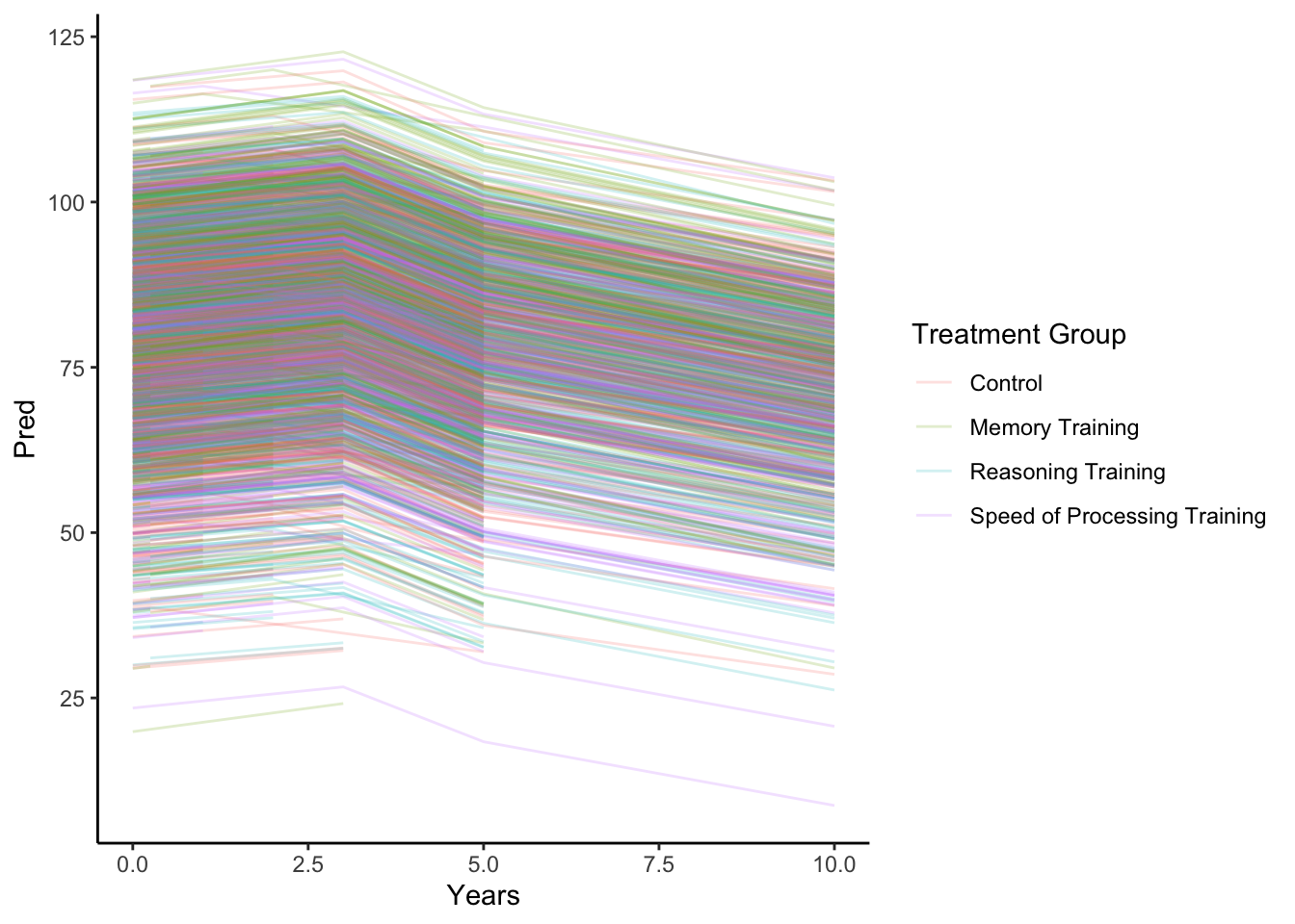
activeLong %>% drop_na(Memory, Years, INTGRP) %>%
  mutate(Pred = predict(mod1, re.form = NA)) %>%
  distinct(Years,INTGRP,Pred) %>%
  ggplot(aes(x = Years, y = Pred, color = INTGRP)) +
  geom_line() +
  labs(color = 'Treatment Group') + theme_classic()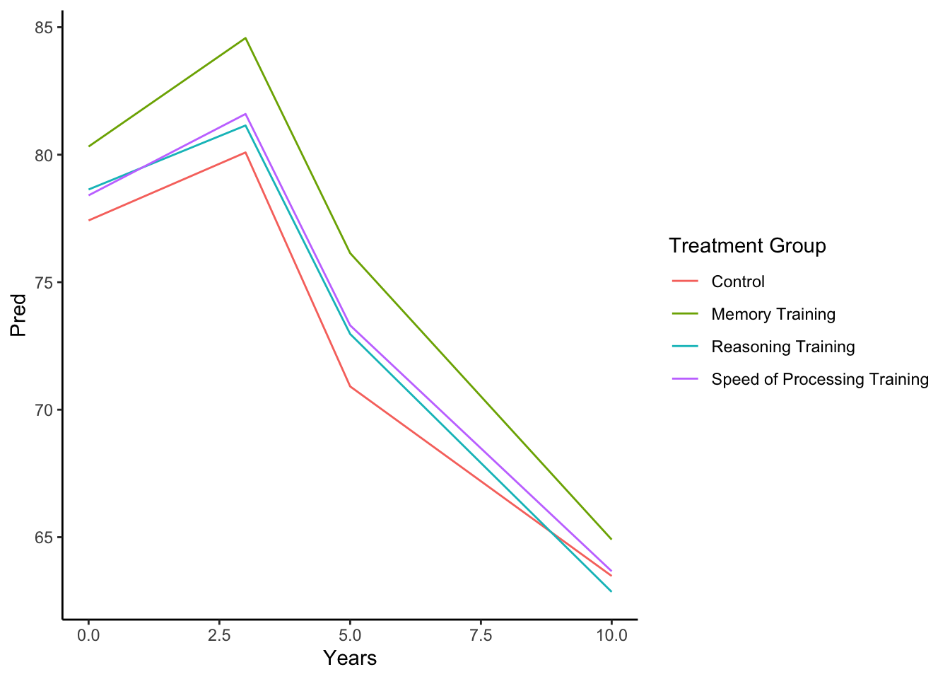
- .
Solution
# Manual Code to get t-values: fixef(mod1)/sqrt(diag(vcov(mod1)))
summary(mod1)
Linear mixed model fit by maximum likelihood ['lmerMod']
Formula: Memory ~ Years * I(Years > 3) * INTGRP + (1 | AID)
Data: .
AIC BIC logLik -2*log(L) df.resid
99505.8 99640.6 -49734.9 99469.8 13236
Scaled residuals:
Min 1Q Median 3Q Max
-5.6494 -0.5424 0.0318 0.5753 6.6810
Random effects:
Groups Name Variance Std.Dev.
AID (Intercept) 255.9 15.997
Residual 56.6 7.524
Number of obs: 13254, groups: AID, 2785
Fixed effects:
Estimate Std. Error
(Intercept) 77.42116 0.64396
Years 0.88896 0.14181
I(Years > 3)TRUE 0.92667 0.99204
INTGRPMemory Training 2.89782 0.90857
INTGRPReasoning Training 1.21432 0.90917
INTGRPSpeed of Processing Training 0.98397 0.90865
Years:I(Years > 3)TRUE -2.37598 0.19568
Years:INTGRPMemory Training 0.52983 0.19807
Years:INTGRPReasoning Training -0.05223 0.19823
Years:INTGRPSpeed of Processing Training 0.17503 0.19789
I(Years > 3)TRUE:INTGRPMemory Training 6.12709 1.38875
I(Years > 3)TRUE:INTGRPReasoning Training 3.52266 1.36602
I(Years > 3)TRUE:INTGRPSpeed of Processing Training 3.61827 1.37079
Years:I(Years > 3)TRUE:INTGRPMemory Training -1.28948 0.27340
Years:I(Years > 3)TRUE:INTGRPReasoning Training -0.48388 0.27080
Years:I(Years > 3)TRUE:INTGRPSpeed of Processing Training -0.61670 0.27146
t value
(Intercept) 120.227
Years 6.269
I(Years > 3)TRUE 0.934
INTGRPMemory Training 3.189
INTGRPReasoning Training 1.336
INTGRPSpeed of Processing Training 1.083
Years:I(Years > 3)TRUE -12.142
Years:INTGRPMemory Training 2.675
Years:INTGRPReasoning Training -0.263
Years:INTGRPSpeed of Processing Training 0.884
I(Years > 3)TRUE:INTGRPMemory Training 4.412
I(Years > 3)TRUE:INTGRPReasoning Training 2.579
I(Years > 3)TRUE:INTGRPSpeed of Processing Training 2.640
Years:I(Years > 3)TRUE:INTGRPMemory Training -4.716
Years:I(Years > 3)TRUE:INTGRPReasoning Training -1.787
Years:I(Years > 3)TRUE:INTGRPSpeed of Processing Training -2.272- INTGRPMemory Training (estimate = 2.89782; t = 3.189): At baseline (Years = 0), we estimate that there is a discernible difference between the mean Memory score of those in Memory Training and those in the Control group.
- Years:INTGRPMemory Training (estimate = 0.52983; t = 2.675): In the first years after training (Years < 3), we estimate that there is discernible difference in the rate of change for the mean Memory score of those in Memory Training and those in the Control group. We note a more positive increase in mean Memory for those in the Memory Training as compare to the Control group.
- I(Years > 3)TRUE:INTGRPMemory Training (estimate = 6.12709 ; t = 4.412): We estimate that there is a discernible difference in the “change in intercept” between the Memory training group and the control group, comparing before and after 3 years of follow up.
- Years:I(Years > 3)TRUE:INTGRPMemory Training (estimate = -1.28948; t = -4.716: We estimate that there is a discernible difference in the change in slopes or decline in mean Memory score between the Memory training group and the control group in the years
In fact, we might be interested in the decline after 3 years.
Among the Control Group, we estimate:
- Mean Memory = 77.42 + 0.88896 Years [for Years < 3]
- Mean Memory = (77.42 + 0.92667 ) + (0.88896 - 2.37598) Years = 78.34667 - 1.4870 Years [for Years > 3]
Among the Memory Training Group, we estimate:
- Mean Memory = (77.42 + 2.89782 ) + (0.88896 + 0.52983) Years = 80.31782 + 1.41879 Years [for Years < 3]
- Mean Memory = (77.42 + 0.92667 + 2.89782 + 6.12709) + (0.88896 + 0.52983 - 2.37598 - 1.28948 ) Years = 87.37158 - 2.24667 Years [for Years > 3]
# Calculating Slopes for Four Equations Above
b = fixef(mod1)
L = matrix(c(0,1,rep(0,14),
             0,1,rep(0,4),1,rep(0,9),
             0,1,rep(0,5),1,rep(0,8),
             0,1,rep(0,4),1,1,rep(0,5),1,rep(0,2)), ncol=16, byrow=TRUE)

L%*%b
[,1]
[1,] 0.8889644
[2,] -1.4870120
[3,] 1.4187960
[4,] -2.2466610- .
Solution
mod3 <- activeLong %>% drop_na(Memory,Years,INTGRP) %>%
  lmer(Memory ~ Years*I(Years > 3)*I(INTGRP == 'Memory Training') + (1|AID), data = ., REML = FALSE)

mod4 <- activeLong %>% drop_na(Memory,Years,INTGRP) %>%
  lmer(Memory ~ Years*I(Years > 3) + INTGRP + (1|AID), data = ., REML = FALSE)

anova(mod1, mod4)
Data: .
Models:
mod4: Memory ~ Years * I(Years > 3) + INTGRP + (1 | AID)
mod1: Memory ~ Years * I(Years > 3) * INTGRP + (1 | AID)
npar AIC BIC logLik -2*log(L) Chisq Df Pr(>Chisq)
mod4 9 99517 99584 -49750 99499
mod1 18 99506 99641 -49735 99470 29.227 9 0.0005933 ***
---
Signif. codes: 0 '***' 0.001 '**' 0.01 '*' 0.05 '.' 0.1 ' ' 1anova(mod1, mod3)Data: .
Models:
mod3: Memory ~ Years * I(Years > 3) * I(INTGRP == "Memory Training") + (1 | AID)
mod1: Memory ~ Years * I(Years > 3) * INTGRP + (1 | AID)
npar AIC BIC logLik -2*log(L) Chisq Df Pr(>Chisq)
mod3 10 99504 99579 -49742 99484
mod1 18 99506 99641 -49735 99470 14.384 8 0.07229 .
---
Signif. codes: 0 '***' 0.001 '**' 0.01 '*' 0.05 '.' 0.1 ' ' 1If there were no difference in the relationship with time comparing treatment groups, there is less than a 0.001 chance we’d see this difference between these models or larger than we did. We have strong evidence in favor of needing an interaction term for treatment group. Thus, we have strong evidence that those in the memory training (or any training) has a difference average mean Memory score pattern over time.
In comparing a model with a simpler Treatment group variable with that of the full group variable, there is not strong evidence to suggest we need the full group variable.
- .
Solution
The BIC also suggests that we choose the model without the interaction term with treatment group. Its addition to the model (added complexity is not balanced by an increased goodness of fit to the data).
BIC(mod1)[1] 99640.65BIC(mod3)[1] 99579.09BIC(mod4)[1] 99584.44- .
Solution
mod5 <- activeLong %>% drop_na(Memory,Years,INTGRP) %>%
  lmer(Memory ~ Years*I(Years > 3)*I(INTGRP == 'Memory Training') + (Years|AID), data = ., REML = FALSE)

BIC(mod3)
[1] 99579.09BIC(mod5)[1] 99062.38This suggests that maybe a model with a subject-specific slope for Years might fit better in terms of correlation better than a random intercept only model.
- .
Solution
activeLong %>% drop_na(Memory, Years, INTGRP) %>%
  mutate(Pred = predict(mod3)) %>%
  mutate(Resid = resid(mod3)) %>%
  ggplot(aes(x = Pred, y = Resid, color = INTGRP)) +
  geom_point(alpha = .2) +
  geom_hline(yintercept = 0) +
  geom_smooth(se = FALSE) +
  theme_classic()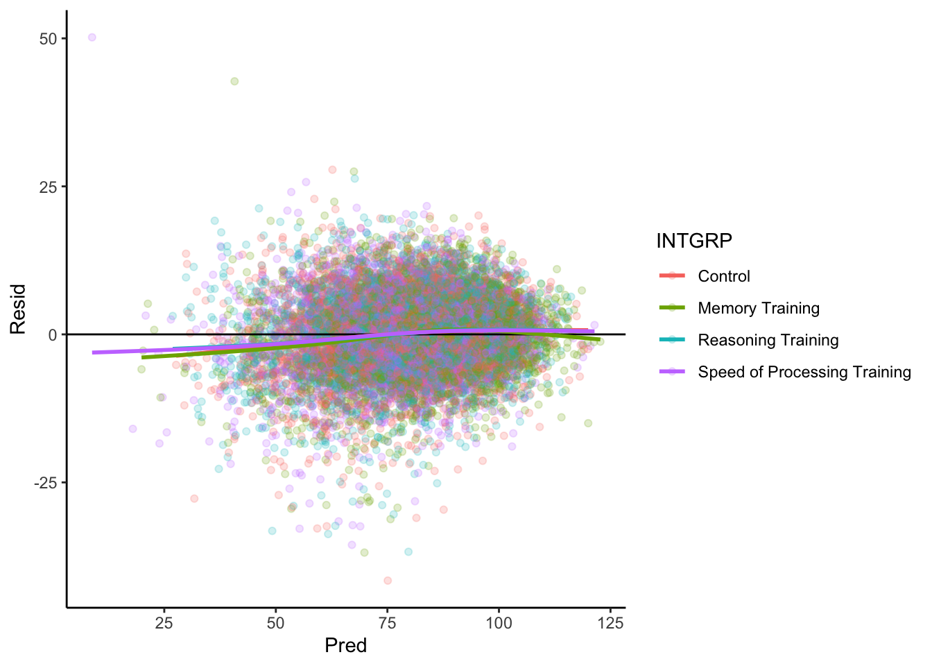
A = ranef(mod3)$AID$`(Intercept)`
qqnorm(A)
qqline(A)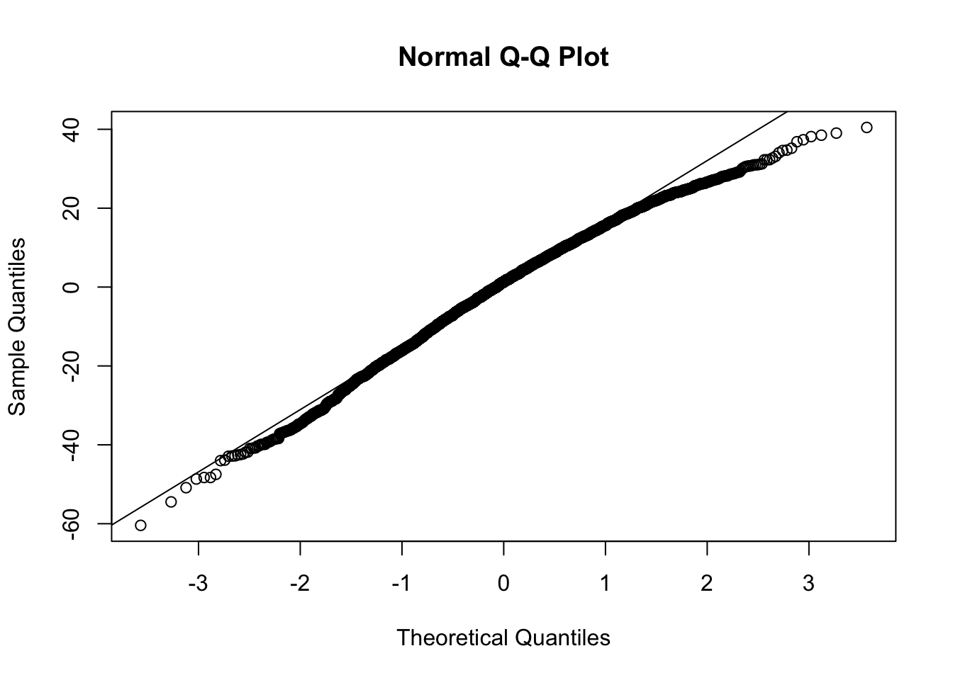
- We constrained the mean model to a piecewise linear (change in relationship at year = 3 from follow up). This is a strong simplifying assumption that we did for interpretation purposes. We could leave Years as
factor(Years)to avoid constraining the relationship over time. - We ended up not including the interaction terms with
INTGRPas they did not improve the model fit that much. With that structure, we assume that the treatment group has the same impact on mean Memory at every time during follow-up. - Lastly we are assuming that the correlation in the data can be modeled with a random intercept model (which is equivalent to the exchangeable correlation structure and constant variance).
- The estimated random intercepts look approximately Normal, so that it good.
Wrap-Up
Finishing the Activity
- If you didn’t finish the activity, no problem! Be sure to complete the activity outside of class, review the solutions in the online manual, and ask any questions on Slack or in office hours.
- Re-organize and review your notes to help deepen your understanding, solidify your learning, and make homework go more smoothly!
After Class
Before the next class, please do the following:
- Take a look at the Schedule page to see how to prepare for the next class.