times <- 1:100
D <- as.matrix(dist(times)) #100x100 matrix with values as lags between every possible value

COR <- 0.9^D #correlation

COV <- COR*4 #covariance (multiply by constant variance)

L <- t(chol(COV)) #cholesky decomposition

z <- rnorm(100)
y <- L %*% z #generate 100 correlated values

plot(times, y, type='l') # plot of the realizations of the process4 Modeling Covariance
Settling In
Highlights from Day 3
Random Process
Definition: A collection of random variables, notated as \(\{Y_t\}_{t\in T}\) for a discrete-indexed process or \(\{Y(t)\}_{t\in T}\) for a continuous-indexed process, measuring the same thing indexed by a set \(T\) that often represents time or space.
. . .
Mean Function:
For a random process \(\{Y(t)\}_{t\in T}\), the mean function is
\[\mu_Y(t) = E[Y(t)]\text{ or } E[Y_t]\]
. . .
Autocovariance Function:
For a random process \(\{Y(t)\}_{t\in T}\), the autocovariance function is
\[\Sigma_Y(s,t) = Cov[Y(s),Y(t)] \text{ or } Cov[Y_s,Y_t]\]
. . .
Autocorrelation Function:
For a random process \(\{Y(t)\}_{t\in T}\), the autocorrelation function is
\[\rho_Y(s,t) = Cor[Y(s),Y(t)] = \frac{\Sigma_Y(s,t)}{\sqrt{\Sigma_Y(s,s)\Sigma_Y(t,t)}}\]
. . .
Covariance Matrix:
For a finite discrete-indexed random process \(\{Y_t\}_{t\in \{1,...,m\}}\), the covariance matrix \(\boldsymbol\Sigma\) is a \(m\times m\) matrix with elements
\[\sigma_{ij} = Cov(Y_i,Y_j)\] in the \(i\)th row and \(j\)th column.
. . .
Correlation Matrix:
For a finite discrete-indexed random process \(\{Y_t\}_{t\in \{1,...,m\}}\), the covariance matrix \(\mathbf{R}\) is a \(m\times m\) matrix with elements
\[\rho_{ij} = Cor(Y_i,Y_j) = \frac{Cov(Y_i,Y_j)}{SD(Y_i)SD(Y_j)}\]
in the \(i\)th row and \(j\)th column.
Comparison to Other Sources
Wikipedia on Random/Stochastic Process
Let’s ask GenAI “Give me an overview of a random process.”
Big Picture
Learning Goals
- Explain and illustrate how we can model covariance by constraining a covariance matrix.
- Explain and illustrate how we can model covariance by constraining an autocovariance function.
- Implement covariance model estimation by assuming stationarity (ACF and Semi-Variogram).
Notes: Modeling Covariance
Warm Up
The covariance matrix is a symmetric matrix of all pairwise covariances, organized into a matrix form. The \(ij\)th element (\(i\)th row, \(j\)th column) of the matrix is \(Cov(Y_i,Y_j) = \sigma_{ij}\).
The correlation matrix is a symmetric matrix of all pairwise correlations, organized into a matrix form. The \(ij\)th element (\(i\)th row, \(j\)th column) of the matrix is \(Cor(Y_i,Y_j) = \rho_{ij}\).
Without looking back at your notes,
Come up with a list of properties that have to be true of each \(\sigma_{ij}\) and the covariance matrix \(\boldsymbol\Sigma\).
Come up with a list of properties that have to be true of each \(\rho_{ij}\) and the correlation matrix \(\mathbf{R}\).
Modeling Covariance
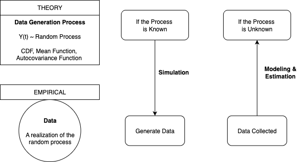
When we have limited data, we won’t be able to estimate all variances and covariances of a random process.
. . .
Thus, we need to make simplifying assumptions and impose constraints in order to empirically estimate variances and covariances from real data (a realization of the process).
. . .
We’ll focus on 3 simplifying assumptions/constraints:
- Weak stationarity (most common with time series)
- Isotropy (strongest assumption, most simplifying, only relevant with spatial data)
- Intrinsic stationarity (weakest assumption, common with spatial data)
Weak Stationarity
A random process is “weakly stationary” (we’ll use just the term stationary) if
- It has a constant mean, \(E[Y(t)] = \mu_Y\)
- It has constant variance, \(Var(Y(t)) = \sigma_Y^2\)
- Covariance is only a function of the difference in time or space
. . .
Autocovariance
If a random process is stationary, we can write the autocovariance function in terms of the difference in time/space, \(h\) (often called a lag).
\[\Sigma_Y(h) = E[(Y_{s+h} - \mu_Y)(Y_{s} - \mu_Y)]\] for any \(s\in T\).
Estimating Autocovariance
Assuming stationarity, we can estimate the autocovariance function with empirical data observations (notice lower case v. upper case) for each lag \(h\),
\[c_h = \frac{1}{n} \sum^{n-|h|}_{t = 1} (y_t - \bar{y})(y_{t+|h|} - \bar{y})\]
In R: acf() does this calculation.
Isotropic
A random process is isotropic if
- It has a constant mean, \(E[Y(t)] = \mu_Y\)
- It has constant variance, \(Var(Y(t)) = \sigma_Y^2\)
- Covariance is only a function of the distance in time or space
- It is only important to distinguish isotropy for spatial data because space is 2 dimensional so the vector difference is not the same as the vector distance
- For time series, time is 1 dimensional so vector difference = vector distance
Intrinsic Stationarity
A random process has intrinsic stationarity if
- \(Var(Y_{s+h} - Y_s )\) depends only on \(h\), the difference in time or space, the lag.
This is a weaker constraint than weak stationarity.
- In other words, weak stationarity implies intrinsic stationarity but not the other way around.
. . .
Semivariogram
If a random process has intrinsic stationarity it may be useful to consider the semivariogram instead of the autocovariance function.
\[\gamma(h) = \frac{1}{2}Var(Y_{s+h} - Y_s )\]
This is more common with spatial data than time series or longitudinal.
Estimating Semivariogram
\[\hat{\gamma}(h_u) = \frac{1}{2 | \{i-j \in H_u \} |} \sum_{\{i-j \in H_u \}}(y_{i} - y_j )\] where \(H_1,...,H_k\) is a partition of the space of possible distances or lags of \(h\) and \(h_u\) is a representative lag or distance in \(H_u\).
In R: gstat::variogram() does this calculation.
Small Group Activity
Download a template Qmd file to start from here.
Theory
As a group, come up with a list of additional properties that have to be true of each \(\sigma_{ij}\) and the covariance matrix if the random process is weakly stationary.
Consider the semivariogram, defined as \(\gamma(i,j) = 0.5 Var(Y_i - Y_j)\). If the random process \(Y_t\) is stationary, what is the relationship between the semivariogram \(\gamma(i,j)\) and the autocovariance function \(\Sigma(i,j) = Cov(Y_i,Y_j)\). Hint: Try to write \(\gamma(i,j)\) in terms of \(\Sigma(i,j)\).
Conceptual Practice
Imagine a random process of length 100 where the constant variance is 4 and the correlation decays such that with lag 1 it is 0.9, with lag 2 it is \(0.9^2\), with lag 3 it is \(0.9^3\), etc.
Sketch the covariance function, assuming stationarity. Label key features.
Sketch the correlation function, assuming stationarity. Label key features.
Artistically illustrate the structure of the covariance matrix. Label key features.
Last time, we generated data from this random process.
What if we generated data based on the previous value? Is this stationary? What is the autocovariance function like? Any intuition? Any guesses? What do you notice?
m <- 100
times <- 1:m
e <- rnorm(m)
x <- rep(0, m)

x[1] <- 1 # initial value

for(i in times[-1]){
  x[i] <- 0.5*x[i-1] + e[i]  # current based on past value plus error
}

plot(times, x, type='l') # plot of the realizations of the process- Without using the functions
acf()orcor(), try to write R code to estimate the autocorrelation function for one of the realized random processes above. Start by breaking the computation down into smaller tasks and then consider R code.
- Without using any variogram function, try to write R code to estimate the semivariogram for one of the realized random processes above. Start by breaking the computation down into smaller tasks and then consider R code.
Solutions
Warm up
Properties of Covariance Matrix
Solution
- Diagonal elements (\(i\)th row, \(i\)th column): \(Var(Y_i) > 0\)
- Off-Diagonal elements: pairwise covariances \(-\infty \leq Cov(Y_i, Y_j) \leq \infty\) where \(i\not= j\)
- Symmetric and Square \(m \times m\) matrix, $ = ^T $
- Positive semi-definite: can perform Cholesky Decomposition; real & positive eigenvalues
- Decompose into \(\mathbf{R}\) and a diagonal variance matrix (HW1)
- Maximum magnitude of Covariance is product of SD
\[ | Cov(Y_i,Y_j) | \leq SD(Y_i)SD(Y_j)\] and if \(Var(Y_i) = Var(Y_j) = Var(Y)\) for all \(i,j\), then
\[ | Cov(Y_i,Y_j) | \leq Var(Y)\]
Properties of Correlation Matrix
Solution
Diagonal elements (\(i\)th row, \(i\)th column): $ Cor(Y_i,Y_i) = 1$ always
Off-Diagonal elements: pairwise covariances \(-1 \leq Cor(Y_i, Y_j) \leq 1\) where \(i\not= j\)
Symmetric and Square \(m \times m\) matrix, $ = ^T $
Positive semi-definite: can perform Cholesky Decomposition; real & positive eigenvalues
Maximum magnitude of Correlation is 1
\[ | Cor(Y_j,Y_j) | \leq 1\]
Small Group Activity
Theory
- .
Solution
- Covariance is a function of difference in time or space: \(\sigma_{ij} = \Sigma(i-j)\)
- Variance is constant \(\sigma_{ii} = \sigma^2\)
- .
Solution
\[\gamma(i,j) = 0.5 Var(Y_i - Y_j)\] \[= 0.5 [Var(Y_i) + Var(Y_j) - 2Cov(Y_i,Y_j)]\] \[= 0.5 [\sigma^2 + \sigma^2 - 2\Sigma(i,j)]\] \[= 0.5 [2\sigma^2 - 2\Sigma(i-j)]\] \[= \sigma^2 - \Sigma(i-j)\]
Thus, if we assume the stronger constraint of weak stationarity (compared to intrinsic stationarity), the semi-variogram is a function of the difference, \(h = i-j\),
\[\gamma(h) = \sigma^2 - \Sigma(h)\]
Conceptual Practice
- .
Solution

- .
Solution

- .
Solution

- .
Solution
Consider:
- Mean over time
- Variance over time
- Covariance over time
No wrong answers here.
- .
Solution
library(dplyr)
library(ggplot2)

# Goal: Average product of distance from means for each lag k
# For each Lag Distance, pull out Pairs of Outcomes of that lag

n <- length(y)

# Find Mean
ybar <- mean(y)

# Calculate Deviations from Mean
ydev <- (y-ybar)

# Get Lag Distances
Dist <- as.matrix(dist(times))

# Use Outer Product to get a matrix of Products of Every Pair
Prods <- ydev %*% t(ydev)

# Use TidyVerse to summarize (average) within groups of lags
CovFun <- tibble(
  h = as.vector(Dist[lower.tri(Dist,diag=TRUE)]),
  Prod = as.vector(Prods[lower.tri(Prods,diag=TRUE)])
) %>%
  group_by(h) %>%
  summarize(Cov = sum(Prod)/n) %>%
  ungroup()

CovFun %>%
  mutate(Var = CovFun$Cov[1]) %>%
  mutate(Cor = Cov/Var) %>%
  ggplot(aes(x = h, y = Cor))  +
  geom_point() +
  geom_line() +
  xlim(c(0,20)) +
  theme_classic()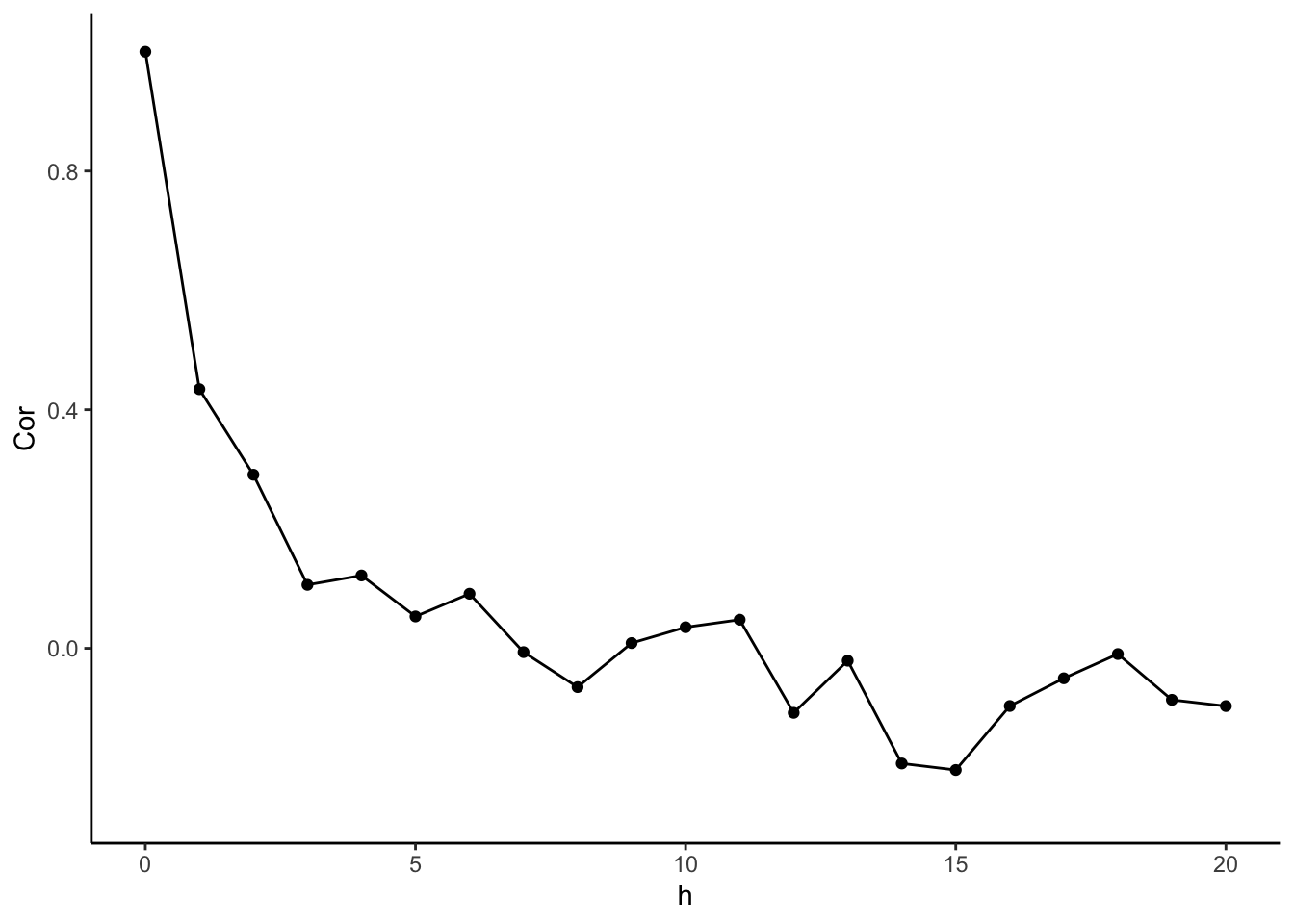
- .
Solution
# For each lag distance, pull out pairs of outcomes of that lag
# Find Variance of differences

# Get Lag Distances
Dist <- as.matrix(dist(times))

#Base R Approach using loops and matrix indices
Vars <- rep(NA, max(Dist) + 1)
for(i in 0:max(Dist)){
  indices <- which(Dist == i, arr.ind = TRUE)
  Vars[i+1] <- 0.5*var(y[indices[,1]]  - y[indices[,2]])
}

Vario <- tibble(
  h = 0:max(Dist),
  V = Vars
)

Vario %>%
  ggplot(aes(x = h, y = V))  +
  geom_point() +
  geom_line() +
  xlim(c(0,20)) +
  theme_classic()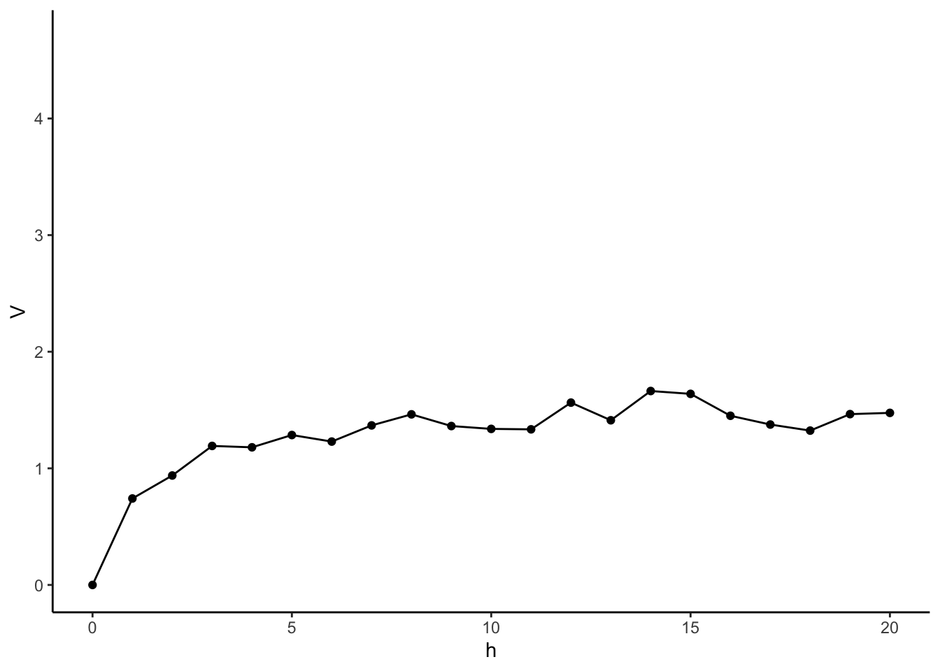
Wrap-Up
Finishing the Activity
- If you didn’t finish the activity, no problem! Be sure to complete the activity outside of class, review the solutions in the online manual, and ask any questions on Slack or in office hours.
- Re-organize and review your notes to help deepen your understanding, solidify your learning, and make homework go more smoothly!
After Class
Before the next class, please do the following:
- Take a look at the Schedule page to see how to prepare for the next class.