15 Intro to Areal Data
Settling In
Learning Goals
- Explain and illustrate the concept of spatial neighbors
- Explain and illustrate the concept of spatial correlation through Moran’s I
- Develop comfort in working with mapping in R (sf package)
Warm Up
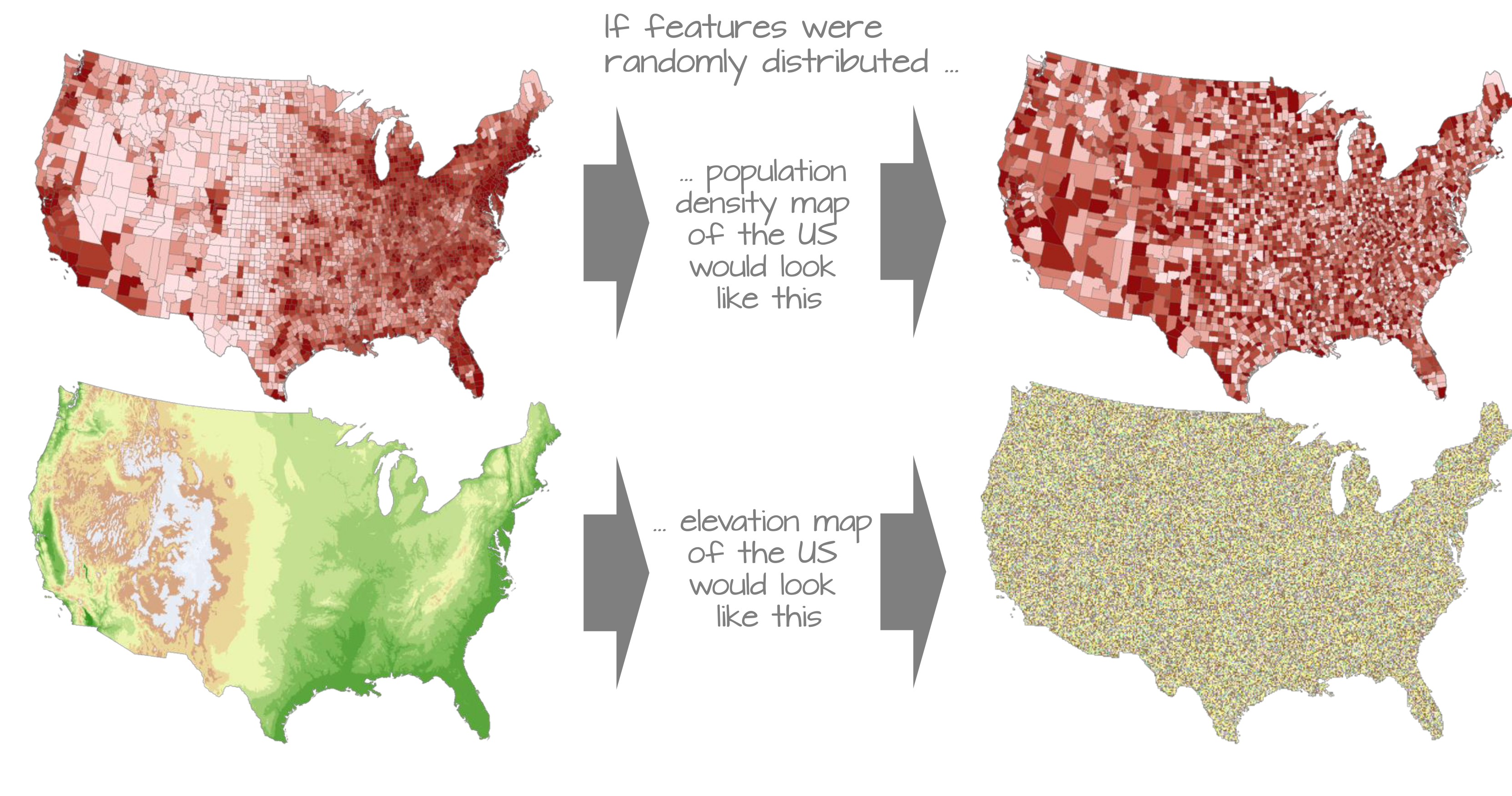
Areal data can often be thought of as a “coarser-resolution” version of other spatial data types, such as
an average/aggregation of point reference data
a count of points within a boundary from a point process.
. . .
Consider your experience with covariance and correlation so far. Discuss:
- What is spatial correlation?
- What does it look like with areal data?
Notes: Areal Data
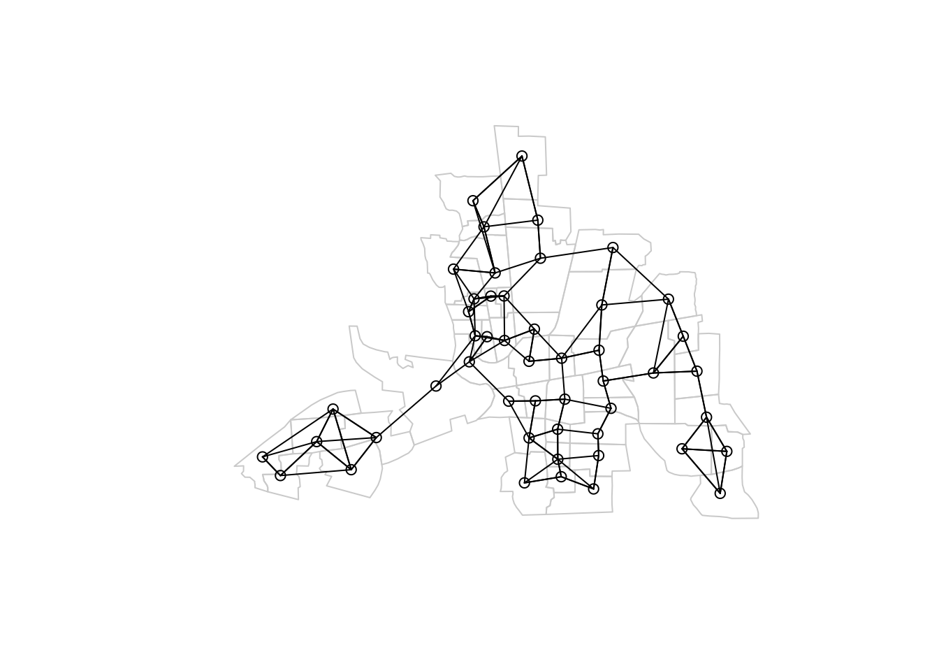
Neighborhoods
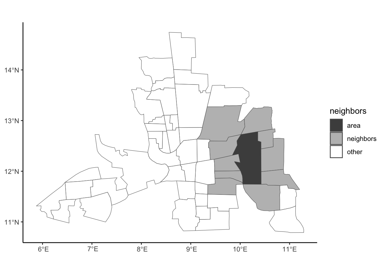
Spatial neighbors are geographic areas that are adjacent or close to each other.
. . .
They can be defined in various ways, such as:
- Contiguity: Two polygons/regions are neighbors if they share a boundary, such as an edge or a corner.
- Queen: If two polygons/regions touch at all, even just at one point, such as a corner, they are neighbors.
- Rook: If two polygons/regions share an edge (more than one point), they are neighbors.
. . .
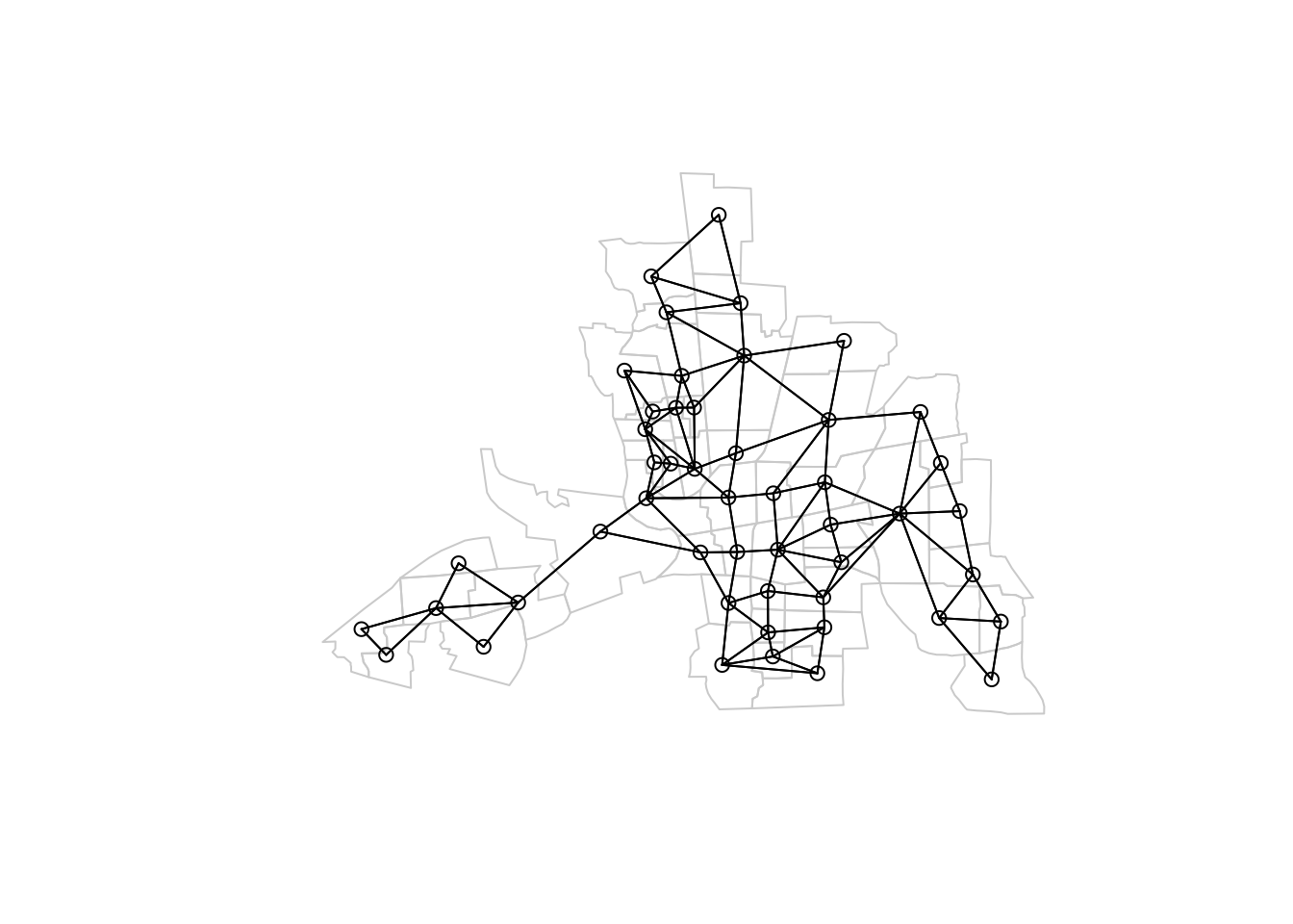
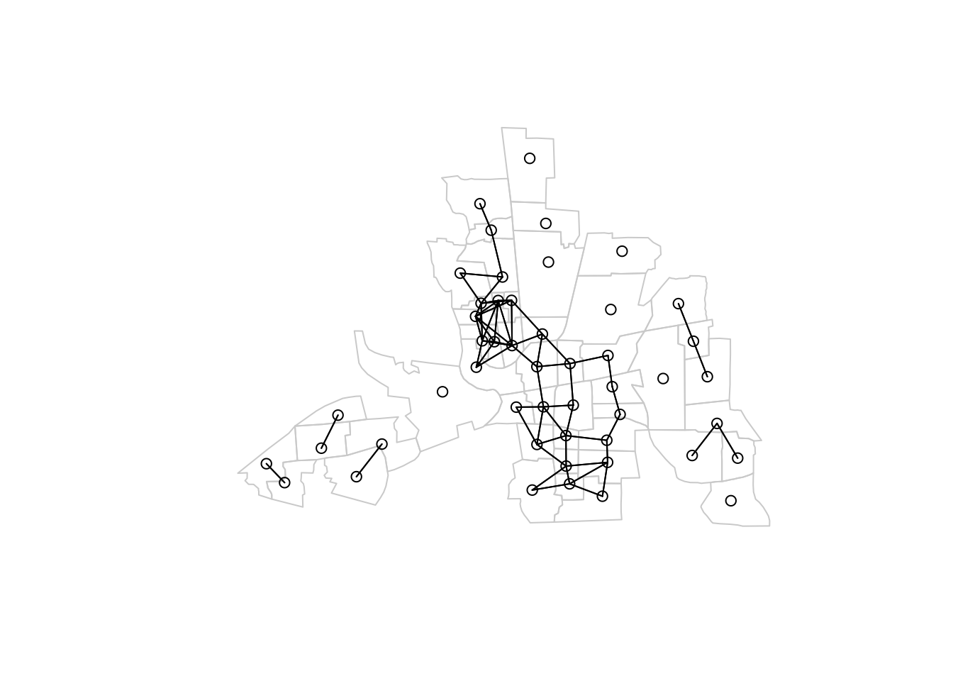
- Distance: Two polygons are neighbors if they are within a certain distance of each other, such as the distance between their centroids (the center points of the polygons/regions).
. . .
- K Nearest Neighbors: Two polygons are neighbors if they are among the K closest polygons/regions based on distance.
See https://mac-stat.github.io/CorrelatedDataNotes/07-spatial.html#neighborhood-structure for more details and code examples.
Weighting Matrix
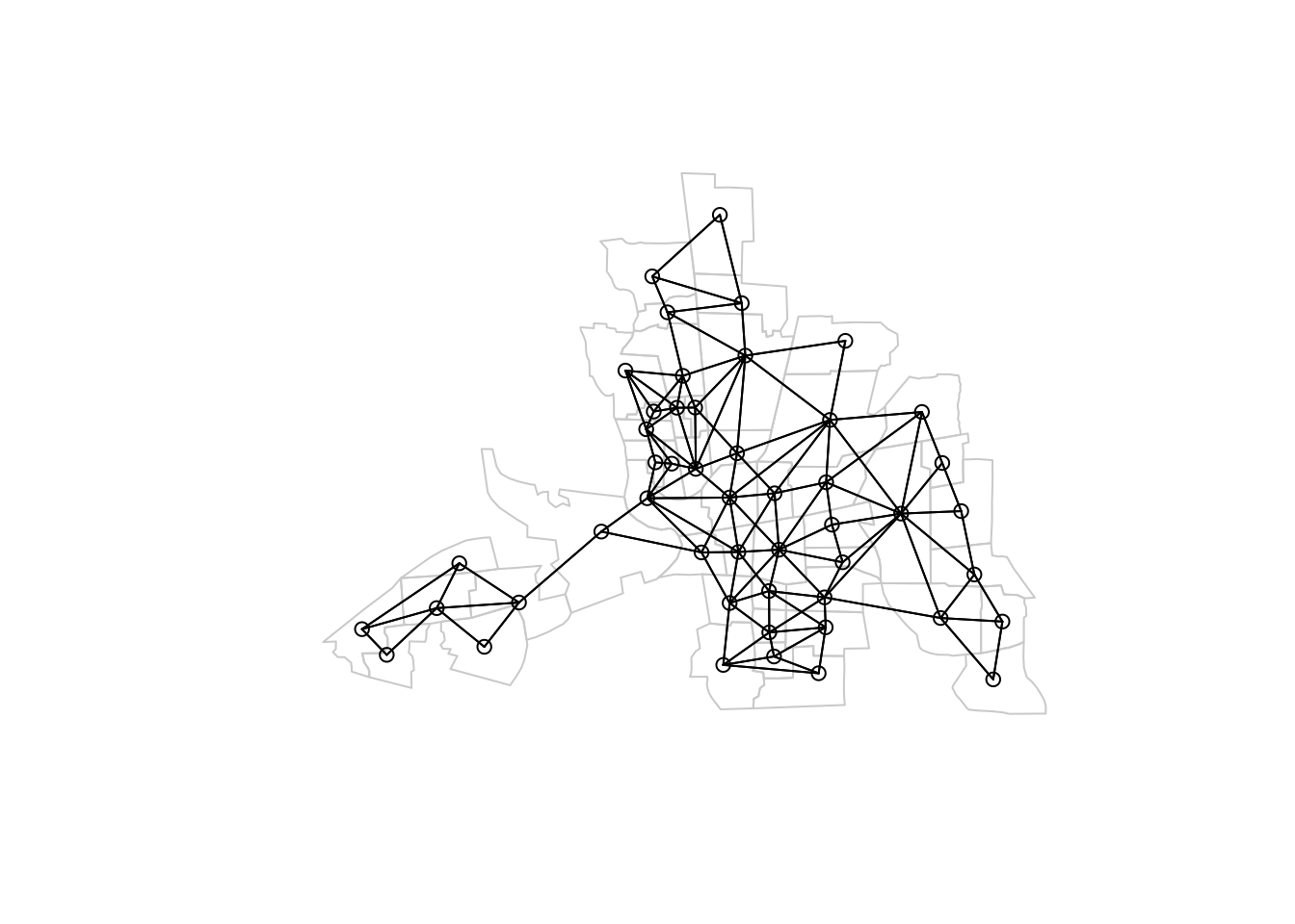
We codify this neighborhood structure with a spatial weighting matrix, \(W\).
- It is also known as an adajency matrix in Graph Theory / Network Science.
. . .
\(W\) is a \(n\times n\) matrix with values of \(w_{ij}\) between 0 and 1.
. . .
- The values can reflect whether or not the \(i\) area is a neighbor of the \(j\) area (0: not neighbor, 1: neighbor)
# Binary W
Mat <- spdep::nb2listw(nb, style = "B") %>% listw2mat()
Mat[1:10,1:10] # here are the first 10 rows and 10 columns...
1 2 3 4 5 6 7 8 9 10
1 0 1 1 0 0 0 0 0 0 0
2 1 0 1 1 0 0 0 0 0 0
3 1 1 0 1 1 0 0 0 0 0
4 0 1 1 0 1 0 0 1 0 0
5 0 0 1 1 0 1 0 1 1 0
6 0 0 0 0 1 0 0 0 1 0
7 0 0 0 0 0 0 0 1 0 0
8 0 0 0 1 1 0 1 0 0 0
9 0 0 0 0 1 1 0 0 0 1
10 0 0 0 0 0 0 0 0 1 0- The values can reflect the strength of the influence of \(i\) on \(j\) (> 0 if there is an influence).
. . .
For example, to account for differing number of neighbors, there are cases in which we row-standardized this 0-1 matrix such that the row sums equal 1.
# Binary W
Mat <- spdep::nb2listw(nb, style = "W") %>% listw2mat()
Mat[1:10,1:10] # here are the first 10 rows and 10 columns...
1 2 3 4 5 6 7 8 9
1 0.0000000 0.50 0.5000000 0.0000000 0.0000000 0.000 0.0000000 0.000 0.000
2 0.3333333 0.00 0.3333333 0.3333333 0.0000000 0.000 0.0000000 0.000 0.000
3 0.2500000 0.25 0.0000000 0.2500000 0.2500000 0.000 0.0000000 0.000 0.000
4 0.0000000 0.25 0.2500000 0.0000000 0.2500000 0.000 0.0000000 0.250 0.000
5 0.0000000 0.00 0.1250000 0.1250000 0.0000000 0.125 0.0000000 0.125 0.125
6 0.0000000 0.00 0.0000000 0.0000000 0.5000000 0.000 0.0000000 0.000 0.500
7 0.0000000 0.00 0.0000000 0.0000000 0.0000000 0.000 0.0000000 0.250 0.000
8 0.0000000 0.00 0.0000000 0.1666667 0.1666667 0.000 0.1666667 0.000 0.000
9 0.0000000 0.00 0.0000000 0.0000000 0.1250000 0.125 0.0000000 0.000 0.000
10 0.0000000 0.00 0.0000000 0.0000000 0.0000000 0.000 0.0000000 0.000 0.250
10
1 0.000
2 0.000
3 0.000
4 0.000
5 0.000
6 0.000
7 0.000
8 0.000
9 0.125
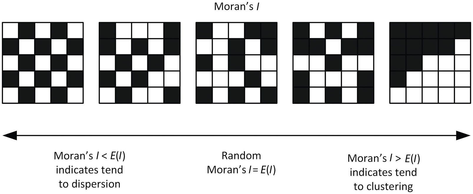
10 0.000Spatial Correlation
Moran’s I, one measure of spatial correlation, is a statistic that quantifies the degree of spatial autocorrelation among neighboring data.
\[I = \frac{n\sum_i\sum_j w_{ij} (Y_i - \bar{Y})(Y_j - \bar{Y})}{\sum_{i,j} w_{ij} \sum_i(Y_i - \bar{Y})^2}\]
. . .
Hypothesis Test for Spatial Independence
\(H_0\): \(Y_i\) are independent and identically distributed, then
\[\frac{I+1/(n-1)}{\sqrt{Var(I)}} \rightarrow N(0,1)\]
. . .
You can calculate a Local version of Moran’s I. For each region \(i\),
\[I_i = \frac{n(Y_i - \bar{Y})\sum_j w_{ij}(Y_j - \bar{Y})}{\sum_{j}(Y_j - \bar{Y})^2}\] such that the global version is proportional to the sum of the local Moran’s I values:
\[I = \frac{1}{\sum_{i\not=j} w_{ij}}\sum_{i}I_i\]
See https://mac-stat.github.io/CorrelatedDataNotes/07-spatial.html#neighborhood-based-correlation for more details and code examples.
Small Group Work
Head to Homework 7. While you should complete it individually, support each other as you work through the examples.
Solutions
Warm Up
Solution
Spatial correlation refers to the relationship between spatially distributed data points, where the value of one point is influenced by the values of nearby points. In areal data, this can be visualized through patterns such as clusters or gradients across geographic areas.
Wrap-Up
Finishing the Activity
- If you didn’t finish the activity, no problem! Be sure to complete the activity outside of class, review the solutions in the online manual, and ask any questions on Slack or in office hours.
- Re-organize and review your notes to help deepen your understanding, solidify your learning, and make homework go more smoothly!
After Class
Before the next class, please do the following:
- Take a look at the Schedule page to see how to prepare for the next class.