2  Probability Review

Settling In

Check in with each other:

• Any issues with tech setup?
• Everyone find HW0 on Moodle?
• Anything brand new to you in video/reading?

No computers needed today! Only paper and pencil.

Everything on the slides is in the online manual: https://bcheggeseth.github.io/452_fall_2025/

Highlights from Day 1

Data Wrangling Time

Date/Time formats in R

• POSIXlt [under the hood: list of vectors with components such as sec, min, hour, mday,mon,year,wday,yday,time zone, daylight savings]
• POSIXct [under the hood: number of seconds since 1970 in UTC time zone]
• Date [under the hood: number of days since 1970-01-01]

. . .

Getting Data into Date/Time formats in R

If the information is stored as a character string, we need to convert it to the POSIXct format

• mdy_hm(), ymd_hm(), ymd(), hms(), etc.
• parse_date_time() for more complicated strings

x <- c("2010-04-14-04-35-59", "2010-04-01-12-00-00")
ymd_hms(x)

[1] "2010-04-14 04:35:59 UTC" "2010-04-01 12:00:00 UTC"

x <- c(20100101120101, "2009-01-02 12-01-02", "2009.01.03 12:01:03",
       "2009-1-4 12-1-4",
       "2009-1, 5 12:1, 5",
       "200901-08 1201-08",
       "2009 arbitrary 1 non-decimal 6 chars 12 in between 1 !!! 6",
       "OR collapsed formats: 20090107 120107 (as long as prefixed with zeros)",
       "Automatic wday, Thu, detection, 10-01-10 10:01:10 and p format: AM",
       "Created on 10-01-11 at 10:01:11 PM")
ymd_hms(x)

 [1] "2010-01-01 12:01:01 UTC" "2009-01-02 12:01:02 UTC"
 [3] "2009-01-03 12:01:03 UTC" "2009-01-04 12:01:04 UTC"
 [5] "2009-01-05 12:01:05 UTC" "2009-01-08 12:01:08 UTC"
 [7] "2009-01-06 12:01:06 UTC" "2009-01-07 12:01:07 UTC"
 [9] "2010-01-10 10:01:10 UTC" "2010-01-11 22:01:11 UTC"

. . .

Getting Components of Date/Time

• hour(), min(), wday(), yday(), mday(), month(), year(), days_in_month(), etc.

. . .

Creating new versions of Date/Time

• Numeric / Decimal Time = hour + minute / 60
• Numeric / Decimal Month and Day = month + day / days_in_month
• Others…

Useful for visualizing while making it accessible to broader public

Watch for…

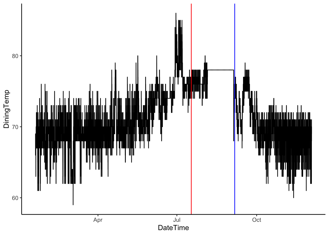
Changes in the Mean

Changes in Variability

Unusual features / anomalies

. . .

Consider the data generating process

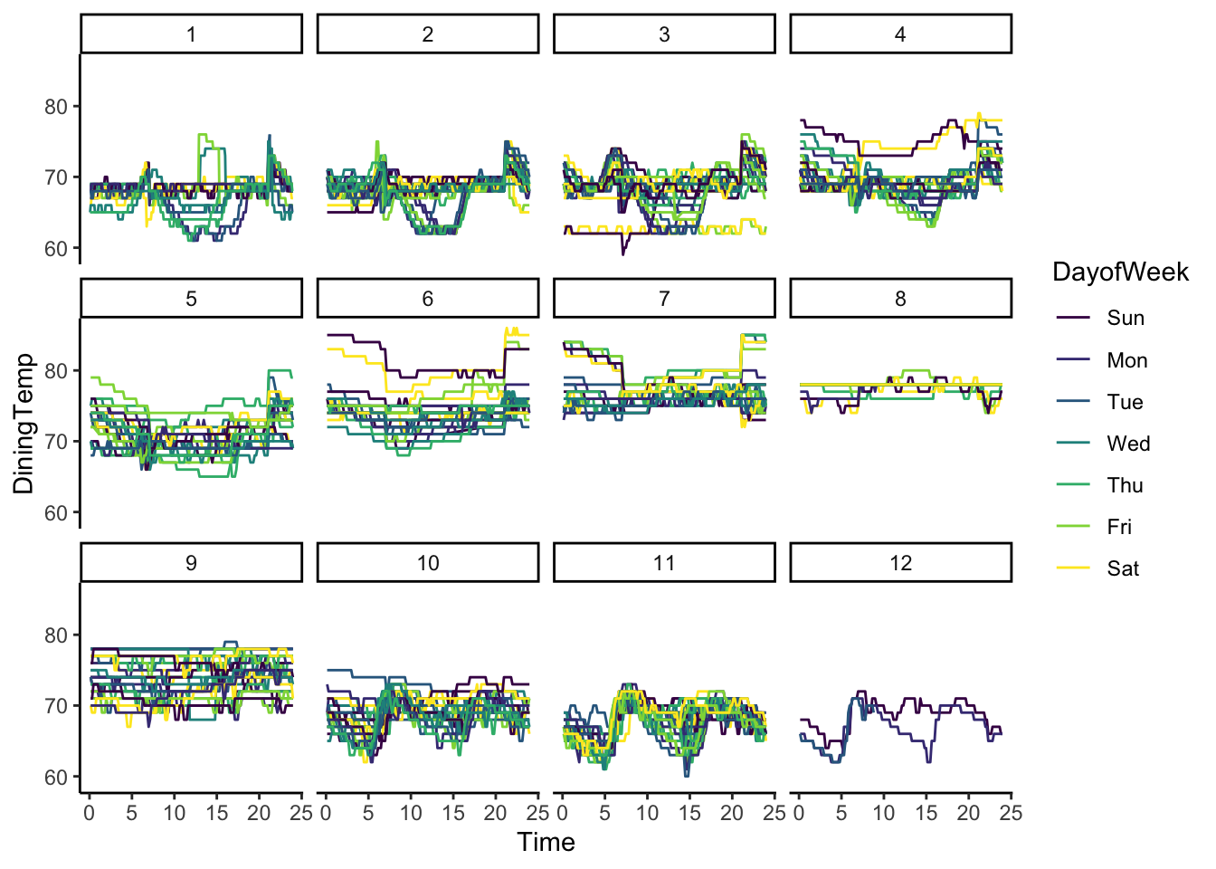
Watch for…

Recurring Patterns

Deterministic Patterns

• Patterns you can explain using the data generating process (weekend v. weekday; winter v. summer; vacations; working outside the house)

. . .

Consider the data generating process

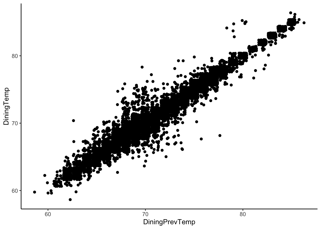
Watch for…

High correlation between lagged observations

Note: I added “jitter” (random noise) to see all of the points since they are all recorded as integers

. . .

Consider modeling this correlation

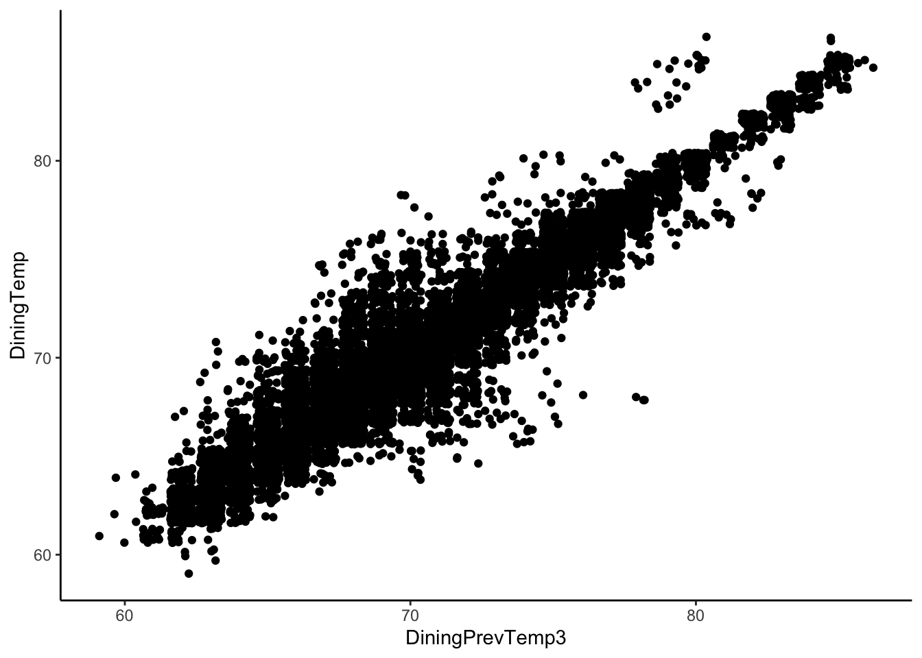
Watch for…

Correlation decreasing in magnitude with larger lags

• Larger lag = further away in time

. . .

Consider how this correlation decays

Learning Goals

• Know the properties of expected value and variance of a random variable.
• Derive mathematical properties of covariance and correlation using properties of expected value and variance.

Probability Review

Probability Warm Up

For a discrete random variable \(X\),

1. How do you calculate the expected value? (definition)

2. List at least two properties of the expected value.

3. How do you calculate the variance? (definition)

4. List at least two properties of the variance.

Review: Covariance

Definition of covariance of two random variables:

\[Cov(X,Y) = E((X - \mu_x)(Y - \mu_y))\]

where \(E(X) = \mu_x\) and \(E(Y) = \mu_y\)

Review: Correlation

Definition of correlation of two random variables:

\[Cor(X,Y) = \frac{Cov(X,Y)}{SD(X)SD(Y)}\]

where \(SD(X) = \sqrt{Var(X)}\) and \(SD(Y) = \sqrt{Var(Y)}\)

Small Group Activity

You are going to prove three REALLY IMPORTANT properties of Covariance!

We’ll need these properties going forward.

Setup

1. Introduce yourselves and check in with each other as humans.

2. Discuss how you want to structure your collaboration. Consider:

• Equitable time with marker
• Equitable contributions to the process (adding to the proof, explaining why you can make the step)
• Whose role it might be to seek resources (Chp 2 in the Notes, asking another group, asking instructor)

Be open and honest about how comfortable you feel about the challenge; support each other in the productive struggle.

Notes:

• If you feel comfortable with the problem, don’t just do it yourself. Talk through strategies/approaches that might be useful; be a guide/coach for the group.
• The goal is that everyone should feel comfortable explaining each step of the proofs.

Challenges

You may assume the properties of expected value (no need to prove those here). You may also assume #1 is true to prove #2 and assume #1 and #2 to prove #3.

1. Prove/show: \(Cov(aX,bY) = ab Cov(X,Y)\) for random variables \(X\) and \(Y\) and constants \(a,b\). Hint: Start with \(Cov(aX,bY)\) and using properties and the definition, rewrite it as \(ab Cov(X,Y)\).

2. Prove/show: \(Cov(X+Y,Z) = Cov(X,Z)+Cov(Y,Z)\) for random variables \(X\), \(Y\), and \(Z\). Hint: Start with \(Cov(X+Y,Z)\) and using properties and the definition, rewrite it.

3. Prove/show: \(Cov(aX+bY,cZ + dW) = acCov(X,Z)+adCov(X,W)+bcCov(Y,Z)+bdCov(Y,W)\) for random variables \(X\), \(Y\), \(Z\), and \(W\). Hint: Start by letting \(V = cZ + dW\).

Solutions

Probability Warm Up

1. Definition of Expected Value

Solution

For a discrete random variable \(X\),

\[E(X) = \sum_{i=1}^{\infty} x_i*P(X = x_i)\]

2. Properties of Expected Value

Solution

For random variables \(X\) and \(Y\) and constant \(a\),

\[E(aX) = \sum_{i=1}^{\infty} ax_i*P(X = x_i) = a\sum_{i=1}^{\infty} x_i*P(X = x_i) = aE(X)\]

\[E(X + a) = \sum_{i=1}^{\infty} (x_i + a)*P(X = x_i) = \sum_{i=1}^{\infty} x_i*P(X = x_i) + a\sum_{i=1}^{\infty} *P(X = x_i) = E(X) + a\]

\[E(X + Y) = \sum_{i=1}^{\infty}\sum_{j=1}^{\infty}(x_i + y_j)*P(X = x_i,Y = y_i)\] \[ =\sum_{i=1}^{\infty}\sum_{j=1}^{\infty}x_i *P(X = x_i,Y = y_i) + \sum_{i=1}^{\infty}\sum_{j=1}^{\infty}y_j*P(X = x_i,Y = y_i) \] \[ =\sum_{i=1}^{\infty}x_i\sum_{j=1}^{\infty}P(X = x_i,Y = y_i) + \sum_{j=1}^{\infty}y_j\sum_{i=1}^{\infty}P(X = x_i,Y = y_i) \] \[ =\sum_{i=1}^{\infty}x_iP(X = x_i) + \sum_{j=1}^{\infty}y_jP(Y = y_i) \] \[ = E(X) + E(Y)\]

3. Definition of Variance

Solution

For a random variable \(X\),

\[Var(X) = E[(X - E(X))^2] \]

Can also be written as:

\[ E[(X - E(X))^2] = E[X^2 - 2XE(X) + (E(X))^2]\] \[= E[X^2] - E[2XE(X)] + E[(E(X))^2]\] \[= E[X^2] - 2E(X)E[X] + (E(X))^2\] \[= E[X^2] - [E(X)]^2 \]

4. Properties of Variance

Solution

For random variables \(X\) and \(Y\) and constant \(a\),

\[Var(aX) = E[a^2X^2] - [E(aX)]^2 = a^2E[X^2]-a^2[E(X)]^2 = a^2Var(X)\]

\[Var(X + a) = E[(X+a - E(X+a))^2] = E[(X+a - E(X)-a)^2] = Var(X)\]

\[Var(X + Y) = E[(X+Y - E(X+Y))^2] \] \[ = E[X+Y - E(X) - E(Y))^2] \] \[ = E[((X - E(X))+(Y - E(Y))^2] \] \[ = E[(X - E(X))^2+(Y - E(Y))^2 + 2(X - E(X))(Y - E(Y))] \] \[ = E[(X - E(X))^2]+E[(Y - E(Y))^2] + 2E[(X - E(X))(Y - E(Y))] \]

\[ = Var(X) + Var(Y) + 2Cov(X,Y)\]

where \(Cov(X,Y) = E[(X - E(X))(Y - E(Y))]\).

Covariance Challenge

1. Prove/show: \(Cov(aX,bY) = ab Cov(X,Y)\) for random variables \(X\) and \(Y\) and constants \(a,b\).

Solution

\[Cov(aX,bY) = E[(aX - E(aX))(bY - E(bY))]\] \[ = E[(aX - aE(X))(bY - bE(Y))]\] \[ = E[ab(X - E(X))(Y - E(Y))]\] \[ = abE[(X - E(X))(Y - E(Y))]\] \[ = ab Cov(X,Y)\]

2. Prove/show: \(Cov(X+Y,Z) = Cov(X,Z)+Cov(Y,Z)\) for random variables \(X\), \(Y\), and \(Z\).

Solution

\[Cov(X+Y,Z) = E[(X+Y - E(X+Y))(Z - E(Z))]\] \[ = E[(X+Y - E(X)-E(Y))(Z - E(Z))]\] \[ = E[((X - E(X))+(Y-E(Y)))(Z - E(Z))]\] \[ = E[(X - E(X))(Z - E(Z))+(Y-E(Y))(Z - E(Z))]\] \[ = E[(X - E(X))(Z - E(Z))]+E[(Y-E(Y))(Z - E(Z))]\] \[ = Cov(X,Z)+Cov(Y,Z)\]

3. Prove/show: \(Cov(aX+bY,cZ + dW) = acCov(X,Z)+adCov(X,W)+bcCov(Y,Z)+bdCov(Y,W)\) for random variables \(X\), \(Y\), \(Z\), and \(W\).

Solution

\[Cov(aX+bY,cZ + dW) = Cov(aX,cZ) + Cov(aX,dW) + Cov(bY,cZ) + Cov(bY,dW)\] \[= acCov(X,Z)+adCov(X,W)+bcCov(Y,Z)+bdCov(Y,W)\]

Wrap-Up

Recap: Variance in Pictures

\[Var(X) = E[(X - E(X))^2] \]

Variance is the average area of the squares

Recap: Covariance in Pictures

\[Cov(X,Y) = E[(X - E(X))(Y - E(Y))]\]

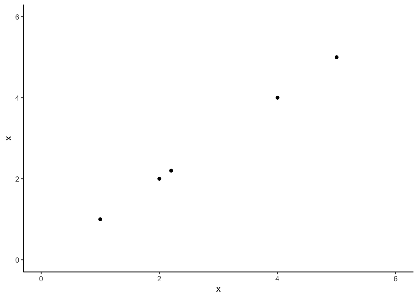
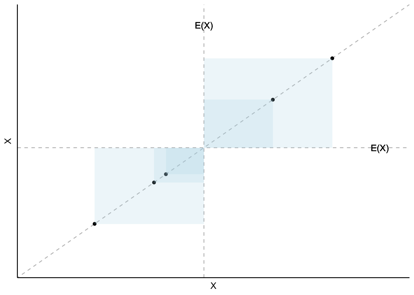
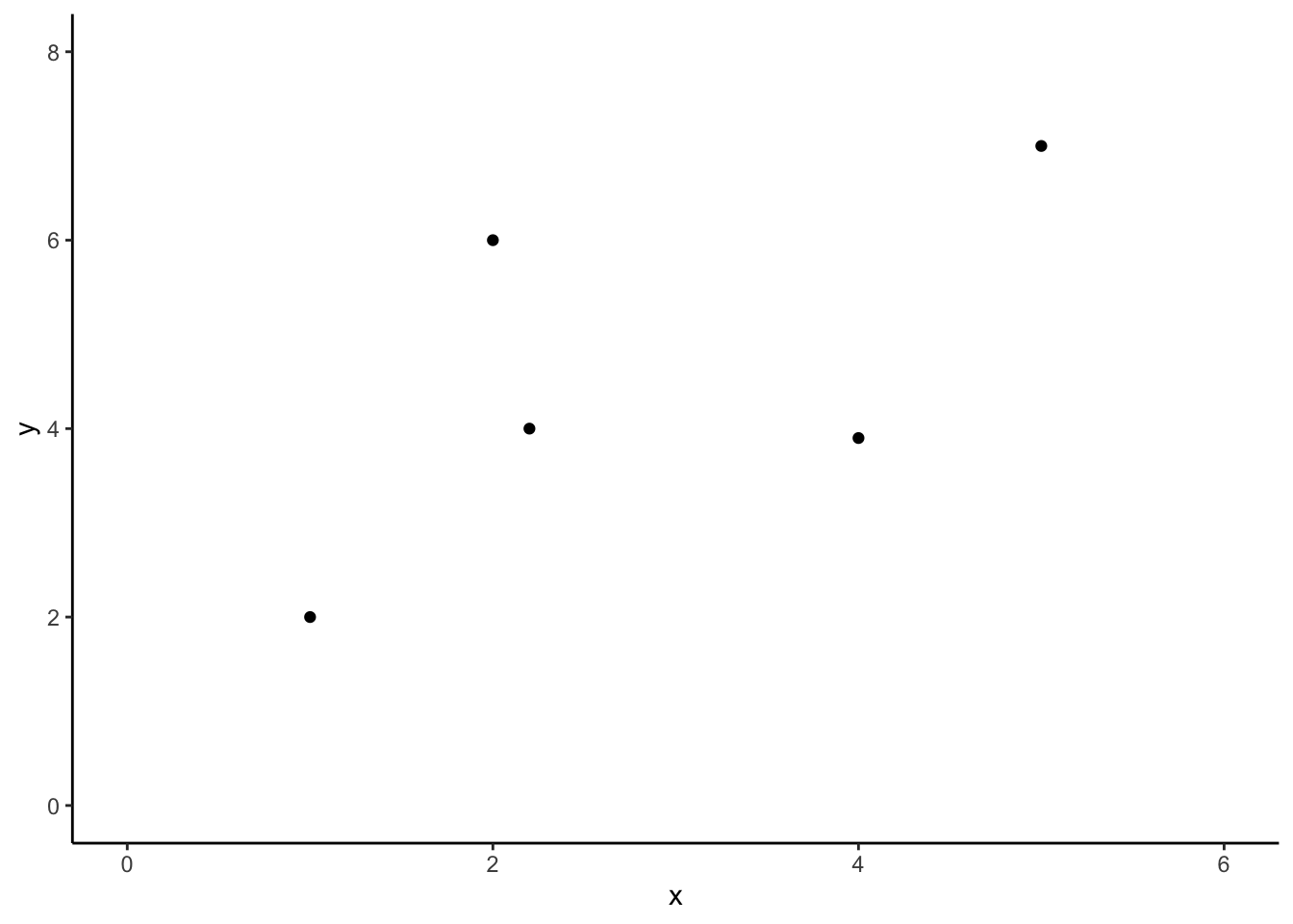
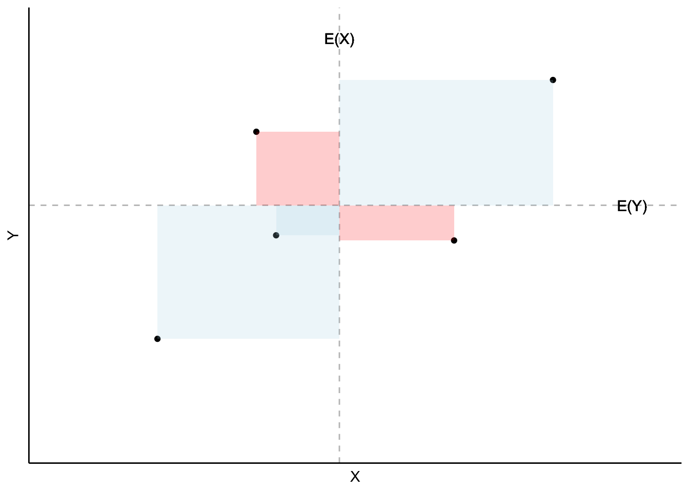
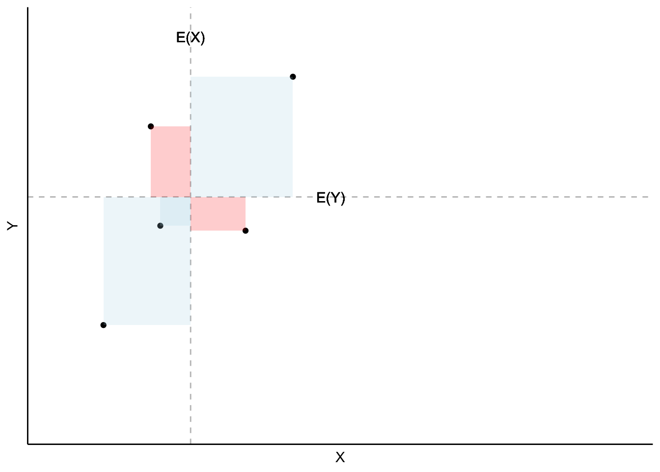
Covariance is the average area of the rectangles (blue + , red -)

Recap: Covariance Properties in Pictures

\[Cov(aX,Y) = aCov(X,Y)\]

Scaling (multiplying by) a random variable by a constant stretches the area of the rectangles proportionally and thus the covariance proportionally

Finishing the Activity

• If you didn’t finish the activity, no problem! Be sure to complete the activity outside of class, review the solutions in the online manual, and ask any questions on Slack or in office hours.
• Re-organize and review your notes to help deepen your understanding, solidify your learning, and make homework go more smoothly!

After Class

Before the next class, please do the following:

• Set up the software and systems we need following these instructions.
• Take a look at the Schedule page to see how to prepare for the next class.