astsa::acf2(y) # estimates and plots ACF and PACF8 ARMA Models
Settling In
Content Conversation 1
Next Thursday, October 2nd!
Overview: In time series mini-project pairs, you’ll meet with Brianna for 15 minutes in her office or the classroom (or on zoom, if needed). For most pairs, this will occur during regularly scheduled class time. During that short time, you and your partner will work together and support each other to communicate your understanding of course content. While you’ll have a partner to work with, you will not have access to any written notes during this conversation.
. . .
Reserve your time: To reserve a time period for you and your partner, go to my Google appointment page and click on a time slot for you and your partner. Please add both names to the name of the calendar event and invite your partner to the Calendar event.
. . .
Why this format: The learning benefit of quizzes and tests comes from the preparation as it provides you an opportunity to stop and synthesize information. This conversation is intended to provide you with this same opportunity in terms of preparation. In contrast to a quiz or test, a conversation more accurately reflects the type of situation you’ll be in in the future where you’ll need to communicate your understanding to others (to convince, to teach, to inform, etc.). I want you to gain more practice in this type of oral communication but with the support of your community, which is why we are doing this in pairs.
. . .
Assessment: I will provide in-the-moment feedback and/or corrections to make sure that you gain the correct conceptual understanding of the statistical topics. I will also share what I observe in terms of collaboration and communication skills to name some areas to work on and further develop. If I do not have an opportunity to share an observation during our time together, I may share that feedback on the individual spreadsheet.
. . .
How to Prepare: Alone and in collaboration with your project partner, I recommend doing the following:
- Review previous material, especially mathematical strategies, properties, and derivations for second moments
- Openly think and discuss how you’ll both make sure the conversation is equitable in terms of time and contribution within the pair of you.
- Openly think and discuss how you want to be supported if you get flustered in the moment.
. . .
Detailed Prompt: In collaboration with your partner and without the use of your notes, walk Brianna through the theoretical derivation of correlation, \(Cor(Y_t, Y_{t-h})\), for an \(MA(q)\) model and discuss the implications of that theory for modeling real data.
Brianna will provide additional details & constraints in the moment to ensure you understand the general process and the reasoning behind the derivation rather than memorizing a set of symbols.
Highlights from Day 7
AR and MA Models
We proved:
MA(1) models are stationary (always)
Theoretical ACF of MA(1) drops to 0 after lag = 1
AR(1) models are stationary as long as \(|\phi_1| < 0\) [Parameter constraints]
Theoretical ACF of AR(1) is exponential decay \(\phi_1^h\)
Mathematical Details
In the notes & in video,
- I discuss important constraints on the coefficients, \(\phi\)’s and \(\theta\)’s
. . .
For an \(AR(p)\) model to be stationary (so that we can write it as \(MA(\infty)\)), we need constraints on \(\phi\)’s
For an \(MA(q)\) model to be invertible (so that we can write it as \(AR(\infty)\)), we need constraints on \(\theta\)’s
. . .
To state these constraints, we need the “backshift operator” \(B\) notation as discussed in video.
This is an optional but recommended depth of understanding.
Learning Goals
- Understand the notation for an ARMA(p,q) and the general mathematical approaches for deriving variance and covariance.
- Explain and implement partial autocorrelation function estimation by assuming stationarity (PACF).
- Explain the common patterns in ACF and PACF for MA(q) and AR(p) models.
- Fit ARMA models to stationary detrended data (also seasonality removed).
Notes: ARMA Models
Recap: AR(p)
\(AR(p)\) Model
\[Y_t = \delta + \phi_1Y_{t-1}+ \phi_2Y_{t-2}+\cdots + \phi_pY_{t-p} + W_t\quad\quad W_t \sim N(0,\sigma^2_w)\]
- Theoretical ACF decays to zero
Recap: MA(q)
\(MA(q)\) Model
\[Y_t = \delta + \theta_1W_{t-1}+ \theta_2W_{t-2}+\cdots + \theta_qW_{t-q} + W_t\quad\quad W_t \sim N(0,\sigma^2_w)\]
- Theoretical ACF drops to zero after \(q\) lags [you’ll provide this in Content Conversation 1]
Partial ACF
Definition: Partial autocorrelation function (PACF) is the autocorrelation function conditional on (i.e. “after accounting for”) observations in between.
\[h_k = \begin{cases} \widehat{Cor}(Y_t,Y_{t-1})\text{ if }k=1\\ \widehat{Cor}(Y_t,Y_{t-k}|Y_{t-1},...,Y_{t-{k-1}})\text{ if }k>1 \end{cases}\]
Note: ACF = PACF for lag = 1 (\(k=1\)).
. . .
Implementation
In R: use astsa::acf2() to estimate and plot ACF and PACF.
. . .
Intuition Building
Example: AR(1), \(\phi_1 = 0.8\), \(\sigma_w = 5\)
set.seed(452)
y <- rep(0, 1000)

y[1] <- rnorm(1, sd = 5)
for(i in 2:1000){
  y[i] <- 0.8 * y[i-1] + rnorm(1, sd = 5) #AR(1) phi_1 = 0.8, sigma_w = 5
}library(tidyverse)
sim <- data.frame(y = y)
sim <- sim %>%
mutate(y_lag1 = lag(y),
y_lag2 = lag(y,2),
y_lag3 = lag(y,3),
y_lag4 = lag(y,4))
# Theoretical ACF for lag 1 = 0.8^1 = 0.8
cor(sim$y, sim$y_lag1, use = 'complete.obs')[1] 0.81267# Theoretical ACF for lag 2 = 0.8^2 = 0.64
cor(sim$y, sim$y_lag2, use = 'complete.obs')[1] 0.6639914# Theoretical ACF for lag 3 = 0.8^3 = 0.512
cor(sim$y, sim$y_lag3, use = 'complete.obs')[1] 0.5406042# Theoretical ACF for lag 4 = 0.8^4 = 0.4096
cor(sim$y,sim$y_lag4, use = 'complete.obs')[1] 0.4353461# Theoretical PACF for lag 1 = ACF for lag 1
cor(sim$y, sim$y_lag1, use = 'complete.obs')[1] 0.81267# Estimating PACF for lag 2 - remove effect of lag 1
lm1 <- lm(y ~ y_lag1, data = sim[-(1:2),])
lm2 <- lm(y_lag2 ~ y_lag1, data = sim[-(1:2),])
# PACF = correlation between residuals of the models above
cor(lm1$residuals, lm2$residuals, use = 'complete.obs')[1] 0.01099112# Estimating PACF for lag 3 - remove effect of lag 1 & 2
lm1 <- lm(y ~ y_lag1 + y_lag2, data = sim[-(1:3),])
lm2 <- lm(y_lag3 ~ y_lag1 + y_lag2, data = sim[-(1:3),])
# PACF = correlation between residuals of the models above
cor(lm1$residuals, lm2$residuals, use = 'complete.obs')[1] -0.007573909astsa::acf2(y)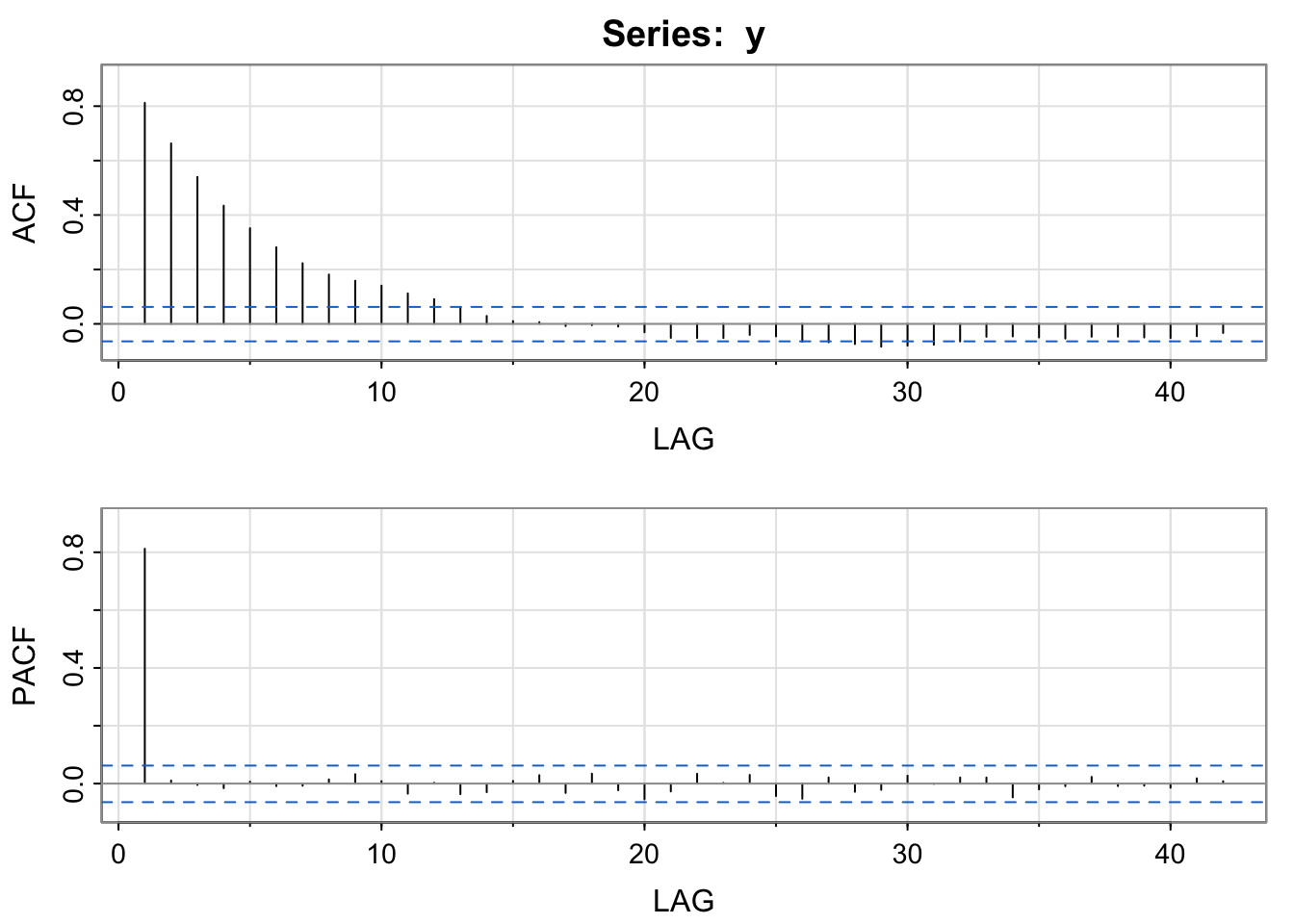
     [,1] [,2] [,3]  [,4] [,5]  [,6]  [,7] [,8] [,9] [,10] [,11] [,12] [,13]
ACF  0.81 0.66 0.54  0.43 0.35  0.28  0.22 0.18 0.16  0.14  0.11  0.09  0.06
PACF 0.81 0.01 0.00 -0.02 0.01 -0.01 -0.01 0.01 0.03  0.01 -0.03  0.00 -0.04
     [,14] [,15] [,16] [,17] [,18] [,19] [,20] [,21] [,22] [,23] [,24] [,25]
ACF   0.03  0.01  0.01 -0.01  0.00 -0.01 -0.03 -0.05 -0.05 -0.05 -0.04 -0.05
PACF -0.03  0.01  0.03 -0.03  0.03 -0.02 -0.05 -0.03  0.03  0.00  0.03 -0.04
     [,26] [,27] [,28] [,29] [,30] [,31] [,32] [,33] [,34] [,35] [,36] [,37]
ACF  -0.07 -0.07 -0.07 -0.08 -0.08 -0.08 -0.06 -0.05 -0.05 -0.05 -0.05 -0.05
PACF -0.05  0.02 -0.03 -0.02  0.03  0.00  0.02  0.02 -0.05 -0.02 -0.01  0.02
     [,38] [,39] [,40] [,41] [,42]
ACF  -0.05 -0.05 -0.05 -0.05 -0.03
PACF -0.01 -0.01 -0.01  0.02  0.01
Review: AR(p)
\(AR(p)\) Model
\[Y_t = \delta + \phi_1Y_{t-1}+ \phi_2Y_{t-2}+\cdots + \phi_pY_{t-p} + W_t\quad\quad W_t \sim N(0,\sigma^2_w)\]
- Theoretical ACF decays to zero
- Theoretical PACF drops to zero after \(q\) lags
Review: MA(q)
\(MA(q)\) Model
\[Y_t = \delta + \theta_1W_{t-1}+ \theta_2W_{t-2}+\cdots + \theta_qW_{t-q} + W_t\quad\quad W_t \sim N(0,\sigma^2_w)\]
- Theoretical ACF drops to zero after \(q\) lags
- Theoretical PACF decays to zero
ARMA Model
Definition: \(ARMA(p,q)\) Model is written as
\[Y_t = \delta + \phi_1Y_{t-1}+ \phi_2Y_{t-2}+\cdots + \phi_pY_{t-p} + W_t + \theta_1W_{t-1}+ \theta_2W_{t-2}+\cdots + \theta_qW_{t-q}\] \[\text{where }W_t \sim N(0,\sigma^2_w)\text{ for all }t\]
Why: With this model, we may be able to model a process with fewer parameters than \(AR(p)\) or \(MA(q)\) alone.
Implementation
In R: fit an \(AR(p)\), \(MA(q)\), or \(ARMA(p,q)\) with the astsa::sarima() function.
sarima(y, p = p, d = 0, q = q)ARMA Model Selection
List of Candidate Models (based on ACF, PACF)
Fit all Candidate Models
Choose amongst Candidate Models
- Double check assumptions of stationarity (Is the trend removed? Is there constant variance?)
- Use training metrics (MSE, AIC, BIC)
- Use hypothesis testing (check coefficients and see if they are distinguishable from 0)
- Use CV metrics (harder to implement with time series – if you do a capstone project in times series, you can try this out; must maintain order of time series)
- Look at residuals of the noise model; want them to be like independent white noise
- Check ACF of residuals and p-values for the Ljung-Box Test – (want large p-values, \(H_0\): residuals are independent white noise)
. . .
You might find auto.arima(). If you can explain to me in fine detail what the function is doing and justify the assumptions it is making, you can use it. If not, don’t use it.
Name that Model
You’ve been selected to participate in our game show called, NAME that MODEL!
Rules of the Game
For each data set, guess AR, MA, or Not Stationary! Then for each, make sure to specify the order of the model.
It may be useful to describe the general patterns you might expect in the estimated ACF for data generated from an AR, MA, or Not Stationary model.
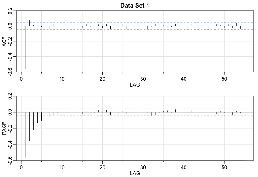
Data set 1
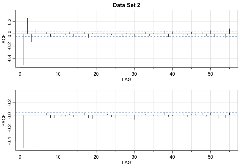
Data set 2
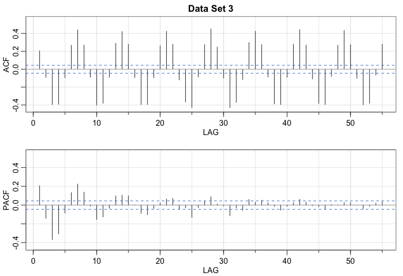
Data set 3
Data set 4
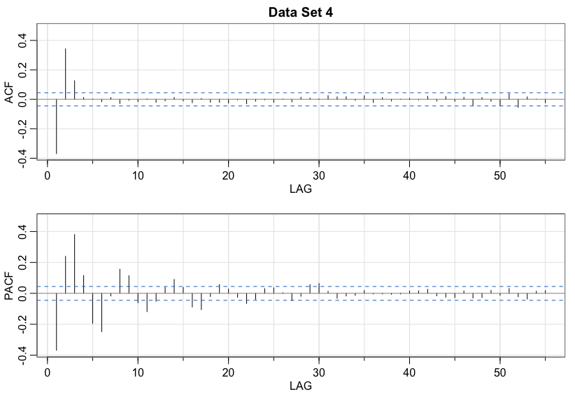
Data set 5
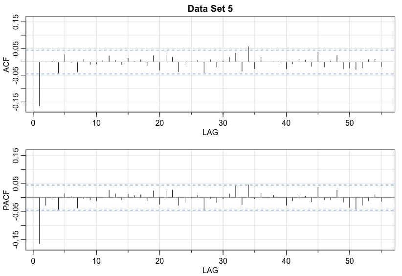
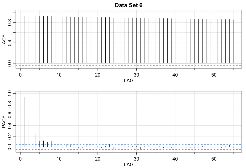
Data set 6
Solutions
Name that Model
You’ve been selected to participate in our game show called, NAME that MODEL!
For each data set, guess AR, MA, or Not Stationary!
Data set 1
Solution
MA(2)Data set 2
Solution
AR(1)Data set 3
Solution
Not StationaryData set 4
Solution
MA(3)Data set 5
Solution
MA(1)Data set 6
Solution
Not StationaryWrap-Up
Finishing the Activity
- If you didn’t finish the activity, no problem! Be sure to complete the activity outside of class, review the solutions in the online manual, and ask any questions on Slack or in office hours.
- Re-organize and review your notes to help deepen your understanding, solidify your learning, and make homework go more smoothly!
After Class
Before the next class, please do the following:
- Take a look at the Schedule page to see how to prepare for the next class.