#Fill in the _ to satisfy the requirements above
rowOne <- c(_,_,_)
rowTwo <- c(_,_,_)
rowThree <- c(_,_,_)

S <- c(rowOne, rowTwo, rowThree)

(Sigma <- matrix(S, byrow=TRUE, nrow=3, ncol=3))3 Random Processes
Settling In
Beyond Mac: Statistics and Data Science Network
a few inspiring people I follow
Highlights from Day 2
Expected Value Properties
For random variables \(X\) and \(Y\) and constant \(a\),
- \(E(aX) = aE(X)\)
- \(E(X + a) = E(X) + a\)
- \(E(X + Y) = E(X) + E(Y)\) which generalizes to
- \(E(\sum_i a_i X_i) =\sum_i a_i E(X_i)\) for a sequence of random variables
. . .
For a \(m\times m\) matrix \(A\) of constants \(a_{ij}\) and random vector \(\mathbf{X} = (X_1,...,X_m)\),
\[E(\mathbf{AX}) = \mathbf{A}E(\mathbf{X})\]
Proof
\[E(\mathbf{AX}) = E\left(\begin{array}{c}a_{11}X_1 + a_{12}X_2+\cdots+a_{1m}X_m\\a_{21}X_1+a_{22}X_2+\cdots+a_{2m}X_m\\ \vdots\\ a_{m1}X_1+a_{m2}X_2+\cdots+a_{mm}X_m\end{array}\right)\] \[= \left(\begin{array}{c}E(a_{11}X_1 + a_{12}X_2+\cdots+a_{1m}X_m)\\E(a_{21}X_1+a_{22}X_2+\cdots+a_{2m}X_m)\\ \vdots\\ E(a_{m1}X_1+a_{m2}X_2+\cdots+a_{mm}X_m)\end{array}\right)\] \[= \left(\begin{array}{c}a_{11}E(X_1) + a_{12}E(X_2)+\cdots+a_{1m}E(X_m)\\a_{21}E(X_1)+a_{22}E(X_2)+\cdots+a_{2m}E(X_m)\\ \vdots\\ a_{m1}E(X_1)+a_{m2}E(X_2)+\cdots+a_{mm}E(X_m)\end{array}\right)\]
\[= \mathbf{A}E(\mathbf{X})\]Covariance (& Variance) Properties
For random variables \(X\), \(Y\), \(Z\) and \(W\) and constants \(a,b,c,d\),
- \(Cov(aX,bY) = ab Cov(X,Y)\)
- Thus follows, \(Cov(aX,aX) = a^2 Cov(X,X) = a^2 Var(X)\)
- \(Cov(aX+bY,cZ + dW) = acCov(X,Z)+adCov(X,W)+bcCov(Y,Z)+bdCov(Y,W)\)
- Thus follows, \(Var(X+Y) = Cov(X+Y,X+Y) = Cov(X,X) + Cov(Y,Y) + 2Cov(X,Y)= Var(X) + Var(Y) + 2Cov(X,Y)\)
For a sequence of random variables \(X_i\) and constants \(a_i\) where \(i\in \{1,2,3,4,5,...\}\),
- this generalizes to \(Cov(\sum_ia_iX_i,\sum_ja_jX_j) = \sum_i\sum_ja_ia_jCov(X_i,X_j)\)
Learning Goals
- Understand mathematical notation used to describe the first and second moments of a sequence of random variables (random process).
- Construct a covariance matrix from a given autocovariance function.
- Generate correlated data from a given covariance matrix.
Notes: Random Process
More details at: https://mac-stat.github.io/CorrelatedDataNotes/03-covariance.html
Random Process
A random process is a series of random variables indexed by time or space, \(Y_t\), defined over a common probability space.
We often collect a finite series of random variables into a random vector \[\mathbf{Y} = \left(\begin{array}{c} Y_{1}\\ Y_{2}\\ \vdots\\\\ Y_{m}\\ \end{array}\right)\]
Autocovariance Function
The autocovariance function of the indices \(s\) and \(t\) in the random process is the covariance of the random variables at those times/spaces,
\[\Sigma_Y(t, s) = Cov(Y_{t}, Y_{s}) = E((Y_t - \mu_t)(Y_s - \mu_s)) = E(Y_sY_t) - \mu_s\mu_t\] where \(\mu_s = E(Y_s)\) and \(\mu_t = E(Y_t)\).
So, if we want the covariance between the 1st and 3rd random variables in the random process,
\[\Sigma_Y(1, 3) = Cov(Y_1,Y_3)\]
Covariance Matrix
The covariance matrix of \(m\) random variables in a random process is one way to organize the variances and covariances.
Note the sigma notation and the relationship with the autocovariance function,
\[\sigma_{ij} = \Sigma_Y(i, j)\]
These \(m(m-1)/2\) unique pair-wise covariances and \(m\) variances can be organized into a \(m\times m\) symmetric covariance matrix,
\[\boldsymbol{\Sigma}_Y = Cov(\mathbf{Y}) = \left(\begin{array}{cccc}\sigma^2_1&\sigma_{12}&\cdots&\sigma_{1m}\\\sigma_{21}&\sigma^2_2&\cdots&\sigma_{2m}\\\vdots&\vdots&\ddots&\vdots\\\sigma_{m1}&\sigma_{m2}&\cdots&\sigma^2_m\\ \end{array} \right) \] where \(\sigma^2_i = \sigma_{ii}\). Note that \(\sigma_{ij} = \sigma_{ji}\).
Correlation
The correlation is a standardized version of the covariance.
The autocorrelation function is
\[\rho_Y(s,t) = \frac{\Sigma_Y(s,t)}{\sqrt{\Sigma_Y(s,s)\Sigma_Y(t,t)}} \]
Note the rho notation,
\[\rho_{ij} = \rho_Y(i, j)\]
These \(m(m-1)/2\) correlations could be organized into a \(m\times m\) symmetric correlation matrix,
\[\mathbf{R}_Y = Cor(\mathbf{Y}) = \left(\begin{array}{cccc}1&\rho_{12}&\cdots&\rho_{1m}\\\rho_{21}&1&\cdots&\rho_{2m}\\\vdots&\vdots&\ddots&\vdots\\\rho_{m1}&\rho_{m2}&\cdots&1\\ \end{array} \right) \]
Note that \(\rho_{ij} = \rho_{ji}\).
Notes: Linear Algebra Review
More details at: https://mac-stat.github.io/CorrelatedDataNotes/appendix-matrix-algebra-review.html
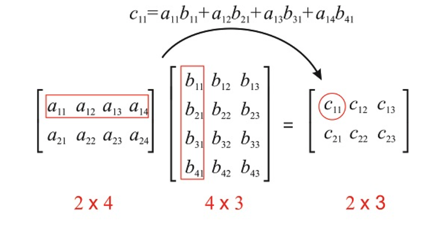
Matrix Multiplication
- Associative Property
\[ \mathbf{A}(\mathbf{B}\mathbf{C}) = (\mathbf{AB})\mathbf{C}\]
- Distributive Property
\[ \mathbf{A}(\mathbf{B} + \mathbf{C}) = \mathbf{AB} + \mathbf{AC}, (\mathbf{A} + \mathbf{B})\mathbf{C} = \mathbf{AC} + \mathbf{BC}\]
- Multiplicative Identity \[\mathbf{I_r A} = \mathbf{AI_c } = \mathbf{A}\] where \(\mathbf{I_r}\) is a \(r\times r\) matrix with 1’s along the diagonal and 0’s otherwise. Generally, we’ll drop the subscript and we’ll assume the dimension by its context.
Matrix Transpose
The transpose of any (\(r\times c\)) \(\mathbf{A}\) matrix is the (\(c \times r\)) matrix denoted as \(\mathbf{A}^T\) or \(\mathbf{A}'\) such that \(a_{ij}\) is replaced by \(a_{ji}\) everywhere.
A matrix is square if \(c=r\). The diagonal of a square matrix are the elements of \(a_{ii}\) and the off-diagonal elements of a square matrix are \(a_{ij}\) where \(i\not=j\).
If \(\mathbf{A}\) is symmetric, then \(\mathbf{A} = \mathbf{A}^T\).
For any matrix \(\mathbf{A}\), \(\mathbf{A}^T\mathbf{A}\) will be a square matrix.
\[(\mathbf{AB})^T = \mathbf{B}^T\mathbf{A}^T\]
\[(\mathbf{A}+\mathbf{B})^T = \mathbf{A}^T+\mathbf{B}^T\]
Homework 1
1a. Prove \[\boldsymbol{\Sigma} = E((\mathbf{X} - E(\mathbf{X}))(\mathbf{X} - E(\mathbf{X}))^T)\] gives a covariance matrix for \(\mathbf{X} = (X_1,X_2)\).
1b. Prove \[\boldsymbol{\Sigma} =\mathbf{V}^{1/2}\mathbf{R} \mathbf{V}^{1/2}\] where \(\mathbf{V}^{1/2}\) gives a covariance matrix for \(\mathbf{X} = (X_1,X_2)\).
Prove \(Cov(\mathbf{AX}) = \mathbf{A}Cov(\mathbf{X})\mathbf{A}^T\).
Prove: If \(X_l\) and \(X_j\) are independent, then \(Cov(X_l, X_j) = 0\). Do so for both discrete RV and continuous RV.
Notes: Generating Data from a Random Process
One way to generate correlated data, one realization of a random process, is to use the Cholesky decomposition of a known covariance matrix of that random process.
Cholesky Decomposition
Cholesky Decomposition: For a real-valued symmetric positive definite matrix \(\mathbf{A}\), it can be decomposed as \[\mathbf{A} = \mathbf{L}\mathbf{L}^T \] where \(\mathbf{L}\) is a lower triangular matrix with real and positive diagonal elements.
A symmetric matrix \(\Sigma\) is positive definite if \[\mathbf{a}^T\mathbf{\Sigma a}>0\] for all real-valued vectors \(\mathbf{a}\not= \mathbf{0}\). If a matrix is positive definite, then all of the eigenvalues will be positive.
Theorem: All valid covariance matricies are positive semi-definite.
Proof
A symmetric matrix \(\Sigma\) is positive semi-definite if \[\mathbf{a}^T\mathbf{\Sigma a}\geq 0\] for all real-valued vectors \(\mathbf{a}\not= \mathbf{0}\).
The covariance matrix \(\Sigma_Y\) of the random vector \(\mathbf{Y}\) of length \(m\) is written as
\[\Sigma_Y = E((\mathbf{Y} - E[\mathbf{Y}])(\mathbf{Y} - E[\mathbf{Y}])^T]\] For an arbitrary real column vector \(\mathbf{a} \in \mathbb{R}^m\),
\[\mathbf{a}^T\Sigma_Y\mathbf{a} = \mathbf{a}^TE((\mathbf{Y} - E[\mathbf{Y}])(\mathbf{Y} - E[\mathbf{Y}])^T]\mathbf{a}\] Due to the linearity of expected value,
\[ = E(\mathbf{a}^T(\mathbf{Y} - E[\mathbf{Y}])(\mathbf{Y} - E[\mathbf{Y}])^T\mathbf{a}]\] Define a new random variable (\(1\times 1\)), \(Z= \mathbf{a}^T(\mathbf{Y} - \mu_Y)\) where \(\mu_Y = E[\mathbf{Y}]\).
Then, we can write
\[\mathbf{a}^T\Sigma_Y\mathbf{a} = E(Z^2)\] Because \(E(Z^2) \geq 0\), we know that
\[\mathbf{a}^T\Sigma_Y\mathbf{a}\geq 0\]
Small Group Activity
Download a template Qmd file to start from here.
Covariance Matrices
- Create a 3x3 symmetric covariance matrix that is has constant variance over time and the covariance is the same when lag, the distance in time, is the same.
- Make sure that the covariance matrix is positive semi-definite by trying the Cholesky Decomposition. If you get an error, go back to #1 and make sure that your covariance matrix satisfies the stated conditions (and the general conditions for variance and covariance).
#chol() gives you upper triangular matrix R such that Sigma = t(R) %*% R
L <- t(chol(Sigma)) # we want lower triangular matrix L such that Sigma = L %*% t(L)
L

L %*% t(L) #double check it gives you Sigma back!
Generating Random Process
- Now generate three random values that are correlated, according to your specified covariance matrix from above. Can you tell these three values are correlated? What might you need to do convince yourself that these are correlated in the way you specified above?
ANSWER:
z <- rnorm(3)
L %*% z # matrix multiplication- Now, let’s generate a random process of length 100 where the constant variance is 4 and the correlation decays such that with lag 1 it is 0.9, with lag 2 it is \(0.9^2\), with lag 3 it is \(0.9^3\), etc.
If we assume that the covariance only depends on the distance in time indices (lags), then we can estimate the covariance as a function of that distance in time indices (lags). Does the estimated covariance look like what you’d expect? Explain what features you were expecting.
times <- 1:100
D <- as.matrix(dist(times)) #100x100 matrix where values are lags between every possible value

COR <- 0.9^D #correlation

COV <- COR*4 #covariance (multiply by constant variance)

L <- t(chol(COV)) #Cholesky decomposition

z <- rnorm(100)
x <- L %*% z #generate 100 correlated values

acf(x, type = 'covariance') #estimated covariance based on distance in time index

acf(x) #estimated correlation based on distance in time index- Repeat the process of generating a random process of 100 observations but change the correlation at distance of 1 index ( = 1 lag) to something other than 0.9 and see how that impacts the estimated covariance and correlation. What changes?
- Then repeat the process of creating a random process and increase the length of the series. How does that impact the estimated covariance and correlation functions?
- Is there any particular material from the probability review section that you’d like us to spend more time on in class? Discuss with your table. Come up with a list of topics; add to #prob-theory Slack channel.
Challenge
- Return to #3 and now try to write R code to convince yourself that the 3 data points you generate using that process are actually correlated. In other words, write R code to estimate the covariance and correlation of data generated in this way. Yes, this is purposefully vague. Consider what is needed in order to estimate the covariance.
Solutions
Notes: Random Process
Prove if \(Z \sim N(0,I)\) and \(\Sigma = LL^T\), then \(Cov(LZ) = \Sigma\).
Proof
\[Cov(LZ) = LCov(Z)L^T\] \[= LIL^T\] \[= LL^T = \Sigma\]
Small Group Activity
Covariance Matrix
- .
Solution
Here is one example that works.
rowOne <-c(3,2,1) # diagonal elements must be the same (constant variance)
rowTwo <- c(2,3,2) # must be symmetric Cov(x1,x2) = Cov(x2,x1)
rowThree <- c(1,2,3) # must be banded Cov(x1,x2) = Cov(x2,x3)

S <- c(rowOne,rowTwo,rowThree)

(Sigma <- matrix(S, byrow=TRUE, nrow=3, ncol=3))
[,1] [,2] [,3]
[1,] 3 2 1
[2,] 2 3 2
[3,] 1 2 3- .
Solution
L <- t(chol(Sigma))
L
[,1] [,2] [,3]
[1,] 1.7320508 0.000000 0.000000
[2,] 1.1547005 1.290994 0.000000
[3,] 0.5773503 1.032796 1.264911L %*% t(L) #double check it gives you Sigma back! [,1] [,2] [,3]
[1,] 3 2 1
[2,] 2 3 2
[3,] 1 2 3Generating Correlated Data
- .
Solution
There is no way to tell that these three points are correlated using only these three points. We know theoretically that they are correlated, but we would need more data points generated in the same matter to estimate the correlation between x1 and x2, etc. See Challenge below!
set.seed(452)
z <- rnorm(3)
L %*% z #matrix multiplication
[,1]
[1,] -2.521016
[2,] -1.848865
[3,] 1.189331- .
Solution
The correlation is .9^d where d is the distance in time. So that should decrease to zero as d increases. The covariance at lag 0 should be close to 4 (the variance) and the correlation at lag 0 should be equal to 1.
times <- 1:100
D <- as.matrix(dist(times)) #100x100 matrix with values as lags between every possible value

COR <- 0.9^D #correlation

COV <- COR*4 #covariance (multiply by constant variance)

L <- t(chol(COV)) #Cholesky decomposition

z <- rnorm(100)
x <- L %*% z #generate 100 correlated values

acf(x, type = 'covariance') #estimated covariance based on lags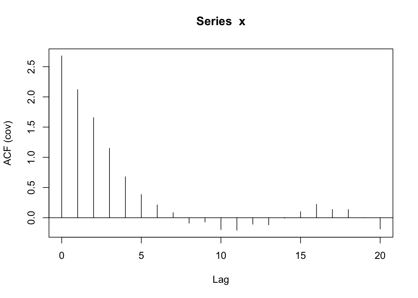
acf(x) #estimated correlation based on lags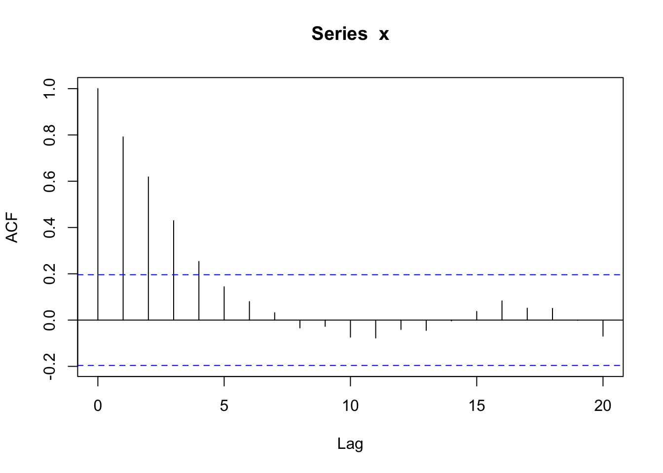
- .
Solution
By changing the correlation at lag 1 to be 0.2 instead of 0.9, the correlation (and covariance) decays to zero faster. There is quite a bit of “noise” with non-zero correlation values at higher lags.
times <- 1:100
D <- as.matrix(dist(times)) #100x100 matrix with values as lags between every possible value

COR <- 0.2^D #correlation

COV <- COR*4 #covariance (multiply by constant variance)

L <- t(chol(COV))

z <- rnorm(100)

x <- L %*% z

acf(x, type = 'covariance') #estimated covariance based on lags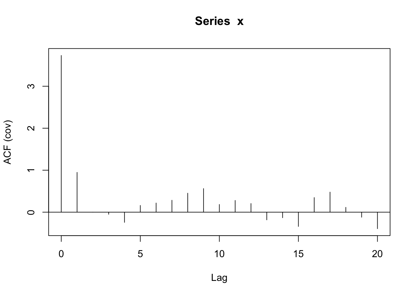
acf(x) #estimated correlation based on lags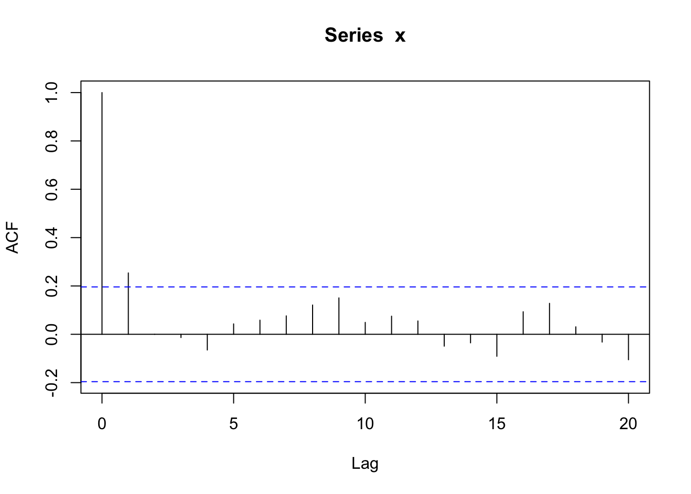
- .
Solution
With more data (increased length of time series), we have more data to estimate the correlation between observations 1 time unit apart, etc. So it should look smoother and less noisy.
times <- 1:1000
D <- as.matrix(dist(times)) #1000x1000 matrix with values as lags between every possible value

COR <- 0.9^D #correlation

COV <- COR*4 #covariance (multiply by constant variance)

L <- t(chol(COV))

z <- rnorm(1000)

x <- L %*% z

acf(x, type = 'covariance') #estimated covariance based on lags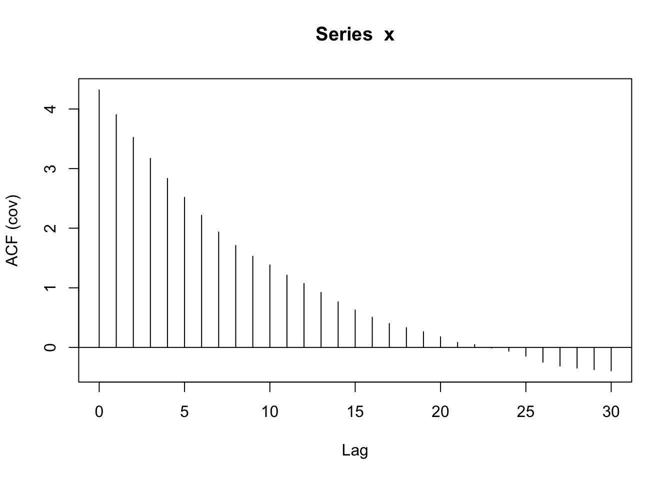
acf(x) #estimated correlation based on lags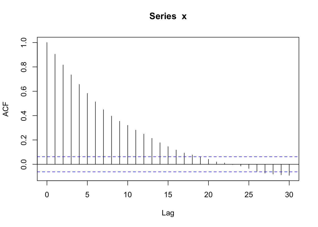
Challenge
- .
Solution
rowOne <-c(3,2,1)
rowTwo <- c(2,3,2)
rowThree <- c(1,2,3)

D <- c(rowOne,rowTwo,rowThree)
Sigma <- matrix(D, byrow=TRUE, nrow=3, ncol=3)
L <- t(chol(Sigma))

x <- matrix(0, ncol = 3, nrow = 5000)

for(i in 1:5000){
  z <- rnorm(3)
  x[i,] <- L %*% z #Generated Correlated Data
}


#Aggregating Across 5000 Realizations
var(x[,1]) #~Var(X1)
[1] 3.023824var(x[,2]) #~Var(X2)[1] 3.086604var(x[,3]) #~Var(X3)[1] 3.058142cor(x[,1],x[,2]) #~Cor(X1,X2)[1] 0.6533786cov(x[,1],x[,2]) #~Cov(X1,X2)[1] 1.996106cor(x[,2],x[,3]) #~Cor(X2,X3)[1] 0.6772473cov(x[,2],x[,3]) #~Cov(X2,X3)[1] 2.080734cor(x[,1],x[,3]) #~Cor(X1,X3)[1] 0.3350164cov(x[,1],x[,3]) #~Cov(X1,X3)[1] 1.018763cor(x) # Estimate Correlation Matrix of repeated measurements of the 3 variables [,1] [,2] [,3]
[1,] 1.0000000 0.6533786 0.3350164
[2,] 0.6533786 1.0000000 0.6772473
[3,] 0.3350164 0.6772473 1.0000000cov(x) # Estimate Covariance Matrix of repeated measurements of the 3 variables [,1] [,2] [,3]
[1,] 3.023824 1.996106 1.018763
[2,] 1.996106 3.086604 2.080734
[3,] 1.018763 2.080734 3.058142# Cor(X,Y) = Cov(X,Y)/SD(X)SD(Y)
# Cov(X,Y) = Cor(X,Y) * SD(X) * SD(Y)
# If Constant Var: SD(X) = SD(Y)
# Cov(X1,X2) = Cor(X1,X2) * Var(X) so Cov(X1,X2) <= Var(X)Wrap-Up
Finishing the Activity
- If you didn’t finish the activity, no problem! Be sure to complete the activity outside of class, review the solutions in the online manual, and ask any questions on Slack or in office hours.
- Re-organize and review your notes to help deepen your understanding, solidify your learning, and make homework go more smoothly!
After Class
Before the next class, please do the following:
- Take a look at the Schedule page to see how to prepare for the next class.
- Work on After Class assignments.