set.seed(452)
y <- vector('numeric', 250) # Pre-allocate memory: generate a vector of missing values
y[1] <- rnorm(1, sd = 1) # Initialization of process (big bang?)

for(i in 2:250){
  #FILL IN

}

df <- tibble(times = 1:250, y = y)

df %>%
  ggplot(aes(x = times, y = y)) +
  geom_line() +
  labs(title = "Random Walk", x = "Time", y = "Value") +
theme_minimal()6 ACF and Random Walk
Settling In
Learning Goals
- Explain and implement covariance and correlation model estimation by assuming stationarity (ACVF, ACF).
- Understand the derivations of variance and covariance for the random walk.
- Generate data from a random walk in R and estimate variance and covariance.
Notes: Review Foundational Ideas
Group Mind Meld
In groups of 2-3, take 10 minutes to discuss the following:
What are the big picture ideas we’ve covered so far?
How does the probability theory connect with the empirical data analysis?
Take notes and be prepared to share ideas with the larger group.
Differencing: To Remove Trend
1st Order Differences: Remove linear trends
Proof: Let’s assume we have a linear trend (and no seasonality) such that the data generating process is:
\[Y_t = b_0 + b_1t + \epsilon_t\]
where \((b_0 + b_1 t)\) is the trend line, and \(\epsilon_t\) is random noise (\(E(\epsilon_t) = 0\)).
. . .
Then, if we take the first order difference, we have:
\[Y_t - Y_{t-1} = (b_0 + b_1t + \epsilon_t) - (b_0 + b_1(t-1) + \epsilon_{t-1}) \]
. . .
Distribute and expand:
\[= b_0 + b_1t + \epsilon_t - b_0 - b_1t + b_1 - \epsilon_{t-1} \]
. . .
Simplify:
\[= b_1 + \epsilon_t - \epsilon_{t-1} \quad \] This is not a function of time, \(t\), so we have removed the linear trend.
. . .
2nd Order Differences: Remove quadratic trends
Proof: Let’s assume we have a quadratic trend (and no seasonality) such that:
\[Y_t = b_0 + b_1t + b_2t^2 + \epsilon_t\]
where \((b_0 + b_1 t + b_2 t^2)\) is the trend line, and \(\epsilon_t\) is random noise (\(E(\epsilon_t) = 0\)).
. . .
Then, if we take the second order difference, we have:
\[(Y_t - Y_{t-1}) - (Y_{t-1} - Y_{t-2}) = (b_1 - b_2^2 + 2b_2t + \epsilon_t - \epsilon_{t-1}) - (b_1 - b_2^2 + 2b_2(t-1) + \epsilon_{t-1} - \epsilon_{t-2}) \]
. . .
Distribute and expand and simplify:
\[= 2b_2 + \epsilon_t - 2\epsilon_{t-1} + \epsilon_{t-2}\] This is not a function of time, \(t\), so we have removed the quadratic trend.
Differencing: To Remove Seasonality
1st Order Seasonal Differences: Removes seasonality if cyclic pattern is the consistent
Proof: Assume you have a cyclic pattern with period \(k\) (length of 1 cycle), such that
\[Y_t = f(x_t) + s_t + \epsilon_t\]
where \(f(x_t)\) is a non-seasonal trend, \(s_t\) is the seasonal component with period \(k\) \((s_t = s_{t-k} = s_{t-2k} = ...)\) and \(\epsilon_t\) is random noise.
. . .
Then a seasonal difference of order \(k\) is defined as:
\[Y_t - Y_{t-k} = (f(x_t) + s_t + \epsilon_t) - (f(x_{t-k}) + s_{t-k} + \epsilon_{t-k})\]
. . .
If we expand, distributed, and simplify:
\[ = f(x_t) + s_t + \epsilon_t - f(x_{t-k}) - s_{t-k} - \epsilon_{t-k}\] \[ = f(x_t) + \epsilon_t - f(x_{t-k}) - \epsilon_{t-k}\]
which has no seasonality component left, effectively removing the seasonality.
See end of Day 5: Model Components activity for examples (theory and simulation).
Small Group Activity
Download a template Qmd file to start from here.
Data Motivation: Marine Diversity during the Phanerozoic
In a 2004 paper, Cornette and Lieberman suggested that marine diversity in the Phanerozoic period (the last 540 million years) follows a random walk.
Data of interest:
- The total number of marine genera during a period of time (new - extinct)
For most of the Phanerozoic period, both CO2 and number of genera roughly followed a random walk up until the last 50-75 million years. This suggests a big change in the late Mesozoic and Cenozoic era.
What is a random walk?! How does this relate to random processes, autocorrelation, and autocovariance?
Source: https://www.pnas.org/content/101/1/187
Random Walk
Let’s get a sense of what they are referring to when they talk about a random walk model.
Imagine that the total number of genera at time \(t\) is equal to the total number of genera in the last time period \(t-1\) plus some random noise (change due to new species coming into existence and other species dying out).
\[Y_t = Y_{t-1} + W_t\quad\quad W_t \stackrel{iid}{\sim} N(0, \sigma_w^2)\]
- Generate one realization of a random walk of length 250 times. Let \(\sigma^2_w = 1\) for now. I’ve laid out some of the structure you need.
Describe the plot of the random walk. What characteristics does it have?
- Estimate the correlation for each lag (difference in times), assuming it is stationary.
Comment on the estimated correlation function. What do you notice?
Based on these two plots (plot of the series and the plot of acf), do you think a random walk is stationary? Is the mean constant? Is there constant variance over time? Is the covariance only a function of the lag?
Generate 500 realizations of a random walk of length 250 times. Let \(\sigma^2_w = 1\) for now. I’ve laid out some of the structure you need.
gen_rand_walk <- function(n = 250, sigma_w = 1) {
  y <- vector('numeric', n) # Pre-allocate memory: generate a vector of missing values
  y[1] <- rnorm(1, sd = sigma_w) # Initialization of life (big bang?)

  for(i in 2:250){
    ## FILL IN
  }
  return(y) # return the generated random walk
}


rep_y <- matrix(NA, nrow = 500, ncol = 250) # Pre-allocate memory for 500 random walks

for(j in 1:500){
  rep_y[j,] <- gen_rand_walk(n = 250, sigma_w = 1)
}- Calculate the mean and variance at each time point (there are 250 time points), averaging over the 500 series (500 realizations) using the function
apply(). Run?applyin console to see documentation. Plot the mean over time and plot the variance over time. With this additional information, do you think that a random walk is stationary?
- Calculate the covariance and correlation matrix for a random walk based on these 500 realizations. Then plot them based on the lag. With this additional information, do you think that a random walk is stationary?
COV <- as.vector(cov(rep_y))
COR <- as.vector(cor(rep_y))

lags <- as.vector(as.matrix(dist(1:250)))

plot(lags, COV, pch='.')

plot(lags, COR, pch='.')- Now use probability theory to confirm what you think. We let
\[Y_t = Y_{t-1} + W_t\quad\quad W_t \stackrel{iid}{\sim} N(0, \sigma_w^2)\]
If we plug in \(Y_{t-1} = Y_{t-2} + W_{t-1}\) into the equation, we get
\[Y_t = Y_{t-2} + W_{t-1} + W_t\]
If we continue this plugging in, we get
\[Y_t = \sum_{i = 1}^t W_i \quad\quad W_i \stackrel{iid}{\sim} N(0, \sigma_w^2)\]
Now, let’s find the first two moments:
\[E(Y_t) = \]
\[Var(Y_t) = \]
\[Cov(Y_t, Y_{t-h}) = \]
Solutions
Foundational Ideas
Big Picture Ideas
Solution
Here are some examples:
- Covariance decreases in magnitude as difference in time/space increases
- In matrix, the Closer to lower left and upper right corners the smaller the value
- Correlated Data structure
- Time series, longitudinal, and spatial (differences) -Covariance/Correlation
- Properties Cov(X,Y)
- Properties of matrix structure (square, symmetric, positive semi-definite)
- Variances on diagonal >= 0
- Covariances off diagonal (real line) but smaller in magnitude than diagonal values
- We can generate Correlated Data!
- Cholesky decomposition
- Based on the previous/past value (neighbors)
- Modeling covariance (constraints)
- Weak stationarity (constant mean & var, cov is function of difference in time/space)
- Banded matrix (toeplitz matrix)
- Covariance Matrix = Var * Correlation Matrix
- Model components
- Data = Trend + Seasonality + Noise
- Estimate and remove trend and seasonality to focus on noise (think of it as a random process)
- Parametric and non-parametric methods are available
- Random process
- Simplifying assumption/constraints: weak stationarity, isotropic, intrinsic stationarity
Connections
Solution
Here are some examples:
Probability Theory
- \(E()\), \(Var()\), \(Cov()\), \(Cor()\) definitions
- \(E(X) = \mu_x =\) sum of value*prob (type of weighted sum)
- \(Cov(X,Y) = E[(X - mu_x)(Y - mu_y)]\)
- \(Cor(X,Y) = Cov(X,Y)/SD(X)SD(Y)\)
- Properties
- \(Cov(AX) = ACov(X)A^T\)
- Random Variable Distribution & how that impacts the data generation
- Model Constraints/Assumptions
Empirical Data
- Messy
- Decomposition into theoretical components (trend, seasonality, errors)
- We don’t know how it was generated!
- We do our best to gain insight from the data
- We make assumptions about the data generation process and then try and estimate aspects (parameters) of the model process
Bridge Between Them
- Apply probability theory to generate correlated data (simulations)!
- Apply a model (constraints on the model for the data generation process) and estimate characteristics of the model based on messy data.
- We can use probability models to predict and provide a measure of our uncertainty about that prediction based on an assumed model.
Small Group Activity
- .
Solution
set.seed(452)
library(tidyverse)
y <- vector('numeric', 250) #generate a vector of missing values
y[1] <- rnorm(1, sd = 1) #initialization of life (big bang?)

for(i in 2:250){
  y[i] <- y[i-1] + rnorm(1, sd = 1)
}

df <- tibble(times = 1:250, y = y)

df %>%
  ggplot(aes(x = times, y = y)) +
  geom_line() +
  labs(title = "Random Walk", x = "Time", y = "Value") +
  theme_classic()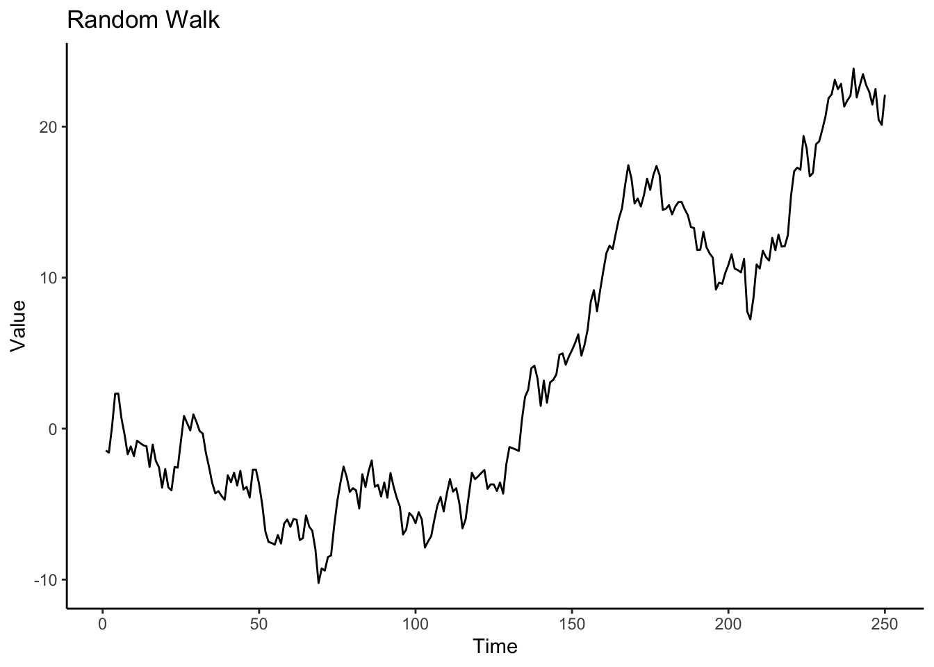
- .
Solution
acf(y)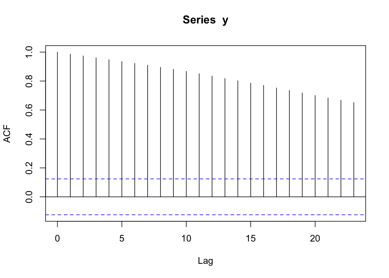
The correlation decreases to zero but is high in magnitude even at large lags.
- .
Solution
It is hard to tell about the mean, the variance, and the covariance from just one realization of the process.
- .
Solution
set.seed(452)
gen_rand_walk <- function(n = 250, sigma_w = 1) {
  y <- vector('numeric', n) # Pre-allocate memory: generate a vector of missing values
  y[1] <- rnorm(1, sd = sigma_w) # Initialization of life (big bang?)

  for(i in 2:250){
    y[i] <- y[i-1] + rnorm(1, sd = sigma_w)
  }
  return(y) # return the generated random walk
}


rep_y <- matrix(NA, nrow = 500, ncol = 250) # Pre-allocate memory for 500 random walks

for(j in 1:500){
  rep_y[j,] <- gen_rand_walk(n = 250, sigma_w = 1)
}- .
Solution
plot(apply(rep_y,2,mean),type='l',ylim=c(-3,3))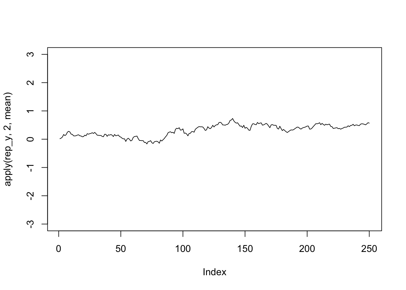
plot(apply(rep_y,2,var),type='l')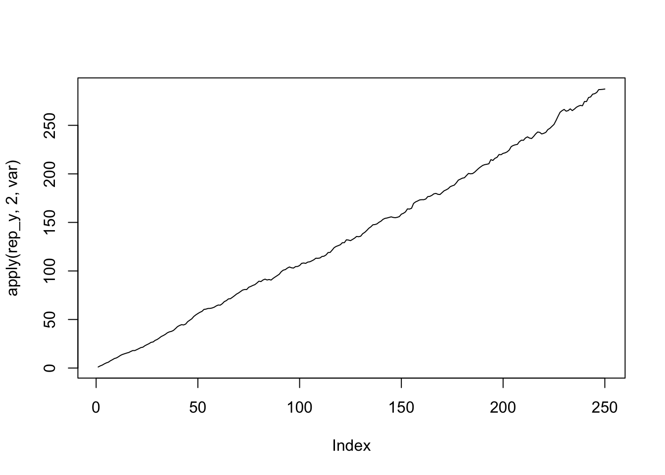
The average over time is close to 0 but the variance increases linearly with time. So no, it is not stationary.
- .
Solution
COV <- as.vector(cov(rep_y))
COR <- as.vector(cor(rep_y))

lags <- as.vector(as.matrix(dist(1:250)))

plot(lags, COV, pch='.')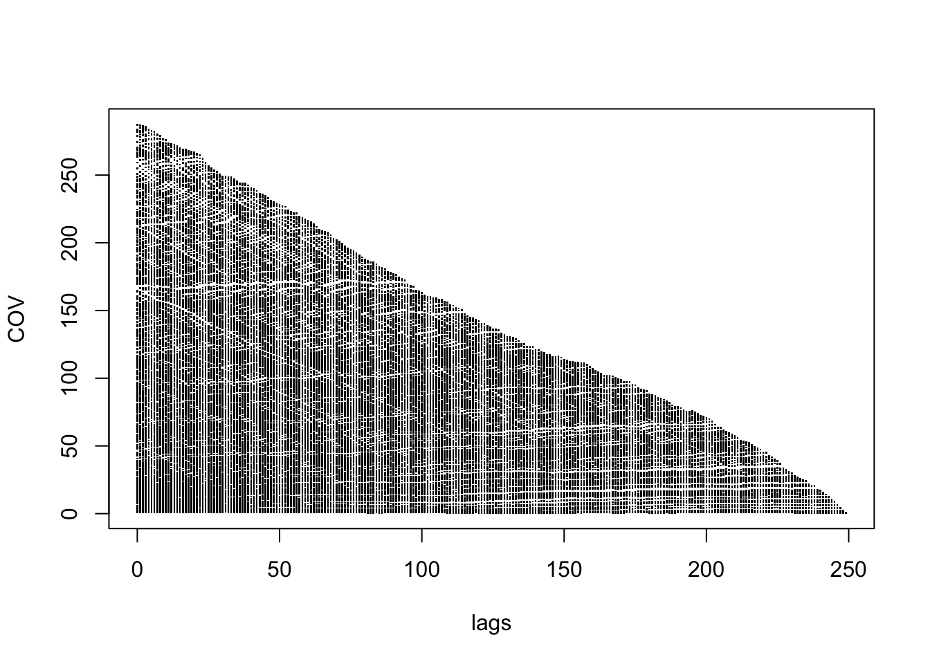
plot(lags, COR, pch='.')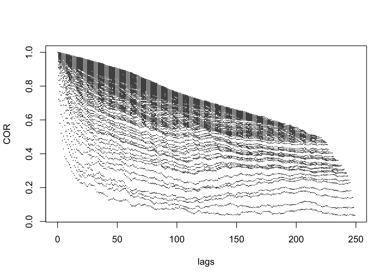
For any given lag, there is a large range of estimated covariances and correlations, so this is further evidence that the random walk is not stationary.
- .
Solution
Now, let’s find the first two moments:
\[E(Y_t) = E(\sum_{i = 1}^t W_i ) = \sum_{i = 1}^t E(W_i) = 0 \] Mean/Expected value is constant
\[Var(Y_t) = Var(\sum_{i = 1}^t W_i ) = \sum_{i = 1}^t Var(W_i) = \sum_{i = 1}^t \sigma_w^2 = t\sigma_w^2\] Variance is NOT constant (increases with time, \(t\))
\[Cov(Y_t, Y_{t-h}) = Cov(\sum_{i = 1}^t W_i, \sum_{i = 1}^{t-h} W_i)\] \[= \sum_{i = 1}^t \sum_{j = 1}^{t-h}Cov( W_i, W_j)\] \[= \sum_{j = 1}^{t-h}Cov( W_j, W_j)\text{ because }Cov(W_i,W_j) = 0\text{ if }j\not=i\] \[= \sum_{j = 1}^{t-h}\sigma_w^2\] \[= (t-h)\sigma_w^2\]
Covariance is NOT only a function of \(h\) (also a function of time, \(t\))
Conclusion: A random walk is NOT stationary.
Wrap-Up
Finishing the Activity
- If you didn’t finish the activity, no problem! Be sure to complete the activity outside of class, review the solutions in the online manual, and ask any questions on Slack or in office hours.
- Re-organize and review your notes to help deepen your understanding, solidify your learning, and make homework go more smoothly!
After Class
Before the next class, please do the following:
- Take a look at the Schedule page to see how to prepare for the next class.