lm(y ~ x, data)11 GLM + GEE
Settling In
Highlights from Day 10
OLS
Definition: Coefficients estimates that minimize the sum of squared residuals from a linear model,
\[\min_{\boldsymbol\beta} (\mathbf{Y} - \mathbf{X}\boldsymbol\beta)^T(\mathbf{Y} - \mathbf{X}\boldsymbol\beta)\] Using calculus and/or linear algebra, we have a closed-form solutions:
\[\hat{\boldsymbol\beta}_{OLS} = (\mathbf{X}^T\mathbf{X})^{-1} \mathbf{X}^T\mathbf{Y}\]
. . .
Properties
- \(E(\hat{\boldsymbol\beta}_{OLS} ) = \boldsymbol\beta\) if the mean model is correct, \(E(\mathbf{Y}) = \mathbf{X}\boldsymbol\beta\)
- Even if \(\mathbf{Y}\) are correlated
- Standard errors are only valid if data is independent
- Stat Theory Folks:
- Assuming \(E(\mathbf{x}_i^T\epsilon_i ) = 0\), \(\hat{\boldsymbol\beta}_{OLS}\) is consistent and asymptotically normal.
- If data is independent, \(\hat{\boldsymbol\beta}_{OLS}\) is BLUE (best linear unbiased estimator).
. . .
Implementation
The OLS estimates of \(\beta\) are the estimates from lm().
. . .
GLS
Definition: Coefficients estimates that minimize the sum of standardized squared residuals,
\[\min_{\boldsymbol\beta} (\mathbf{Y} - \mathbf{X}\boldsymbol\beta)^T\boldsymbol\Sigma^{-1}(\mathbf{Y} - \mathbf{X}\boldsymbol\beta)\] Using calculus, we have a closed-form solution if \(\boldsymbol\Sigma\) is known:
\[\hat{\boldsymbol\beta}_{GLS} = (\mathbf{X}^T\boldsymbol\Sigma^{-1}\mathbf{X})^{-1} \mathbf{X}^T\boldsymbol\Sigma^{-1}\mathbf{Y}\]
. . .
If \(\boldsymbol\Sigma\) is unknown, we have to estimate it from the data, which is what we do in practice.
\[\hat{\boldsymbol\beta}_{GLS*} = (\mathbf{X}^T\hat{\boldsymbol\Sigma}^{-1}\mathbf{X})^{-1} \mathbf{X}^T\hat{\boldsymbol\Sigma}^{-1}\mathbf{Y}\]
. . .
Properties
If \(\boldsymbol\Sigma\) is known,
- Unbiased slope coefficients (estimating the truth on average) if the mean model is correct, \(E(\mathbf{Y}) = \mathbf{X}\boldsymbol\beta\)
- Even if \(\mathbf{Y}\) are correlated
- Standard errors are only valid if we specify the covariance correctly.
- Stat Theory Folks:
- If data is not independent but \(\boldsymbol\Sigma\) is known, \(\hat{\boldsymbol\beta}_{GLS}\) is BLUE (best linear unbiased estimator).
If \(\boldsymbol\Sigma\) is unknown, we estimate it from the data using a working correlation structure and call it feasible GLS.
- Stat Theory Folks:
- Assuming we specify the covariance structure correctly, \(\hat{\boldsymbol\beta}_{GLS}\) is consistent and asymptotically normal.
- This estimate is more efficient than OLS if the non-independent covariance structure is correct.
. . .
Implementation
The feasible GLS estimates of \(\beta\) are the estimates from nlme::gls(),
nlme::gls(y ~ x, data, correlation = corAR1(form = ~ 1 | id)))Learning Goals
- Explain the common model components of a general linear model (GLM)
- Explain the ideas of working correlation models and robust standard error
- Fit GEE models to real data and interpret the output
Generalized Linear Model (GLM)
Definitions
A generalized linear model (GLM) is a generalization of our linear model to non-continuous outcomes
- Linear regression model (continuous outcome)
- Logistic regression model (binary outcome)
- Poisson regression model (count outcome)
. . .
The most common way to estimate the parameters of a GLM is Maximum Likelihood Estimation (MLE)
- What is MLE?!
- It is an optimization procedure for choosing the “best” estimates for the parameters (assuming full distribution).
- The “best” estimates are those that maximize the likelihood of the observed data given the model specification.
- Numerical Optimization Algorithm: Iterative reweighted least squares or Newton’s method are typically used.
- Take Statistical Theory (STAT 355) to learn more!
Model Specification
To specify a GLM model, we need to specify the following:
- Distributional assumption for outcome variable
- Linear: Gaussian/Normal
- Logistic: Binomial
- Poisson: Poisson
- Systematic component
- Choose which explanatory variables (X’s) to be in the model
- Link Function
- Linear: identity
- Logistic: logit
- Poisson: log
See https://mac-stat.github.io/CorrelatedDataNotes/ for more information on GLMs.
Implementation
glm(Y ~ X1 + X2, data = data, family = binomial(link = "logit"))Systematic Component
Y ~ X1 + X2 Distributional & Link Function Assumption
family = binomial(link = "logit")Marginal Models
Definitions
Marginal Models are a type of model that focuses on the average effect of explanatory variables on the outcome, while accounting for correlation between observations within units (e.g., repeated measures on the same subject).
. . .
Generalized Estimating Equations (GEE) is an estimating approach to a Marginal Model when there is natural correlation between observations within unit.
- Linear regression model for longitudinal continuous outcomes
- Logistic regression model for longitudinal binary outcomes
- Poisson regression model for longitudinal count outcomes
. . .
Using GEE to get parameter estimates, we must solve the following estimating equations to get coefficient estimates:
\[0 = \sum_{i=1}^n \frac{\partial \boldsymbol\mu_i}{\partial \boldsymbol\beta }\mathbf{V}_i^{-1}(\mathbf{Y}_i - \boldsymbol\mu_i(\boldsymbol \beta)) \]
where \(\mathbf{Y}_i\) is the vector of outcomes for unit \(i\), \(\boldsymbol\mu_i(\boldsymbol \beta)\) is the vector of expected values for unit \(i\) (defined based on \(\boldsymbol \beta\)), and \(\mathbf{V}_i\) is a working covariance matrix for unit \(i\).
. . .
- When using linear models with continuous outcomes, GEE is similar to GLS.
- Find coefficients that minimize the sum of standardized squared residuals:
\[\min_{\beta} \sum_{i=1}^n (\mathbf{Y}_i - \boldsymbol\mu_i)^T\mathbf{V}_i^{-1}(\mathbf{Y}_i - \boldsymbol\mu_i)\]
where \(\mathbf{V}_i\) is a covariance matrix based on a working correlation structure and \(\boldsymbol\mu_i\) is based on a link function and a linear combination of X variables, \(\mu_{ij} = g^{-1}(\mathbf{x}_{ij}^T\boldsymbol\beta)\),
\[\mathbf{V}_i = \mathbf{A}_i^{1/2} Cor(\mathbf{Y}_i) \mathbf{A}_i^{1/2}\]
where \(\mathbf{A}_i\) is a diagonal matrix with \(Var(Y_{ij} | X_{ij}) = \phi v(\mu_{ij})\) along the diagonal.
Model Specification
To use GEE, we need to specify the following:
- Distributional assumption for outcome variable
- Linear: Gaussian/Normal
- Logistic: Binomial
- Poisson: Poisson
- Systematic component
- Choose which explanatory variables (X’s) to be in the model
- Link Function
- Linear: identity
- Logistic: logit
- Poisson: log
- Working Correlation Structure [NEW]
Properties
Slope coefficients are consistent (i.e. with high probability, our estimates are close to the truth with large data sample sizes) if the mean model is correct
With large sample sizes, we know the sampling distribution of the estimates is approximately Gaussian with \(Cov(\hat{\beta}) = B^{-1}MB^{-1}\) assuming the mean model is correct
\(B^{-1}MB^{-1}\) gives the robust “sandwich” estimator for the coefficient Standard Errors
- Robust in this case means the estimates are valid even if the working correlation structure is wrong
Implementation
mod_gee <- geeM::geem(Y ~ X1 + X2, data = data, family = binomial(link = "logit"), id = id, corstr = "ar1")

summary(mod_gee) #estimates, model SE, robust SE, wald test statistics, p-values
Systematic Component
Y ~ X1 + X2 Distributional & Link Function Assumption
family = binomial(link = "logit")Subject/Unit Identifier
id = idWorking Correlation Assumption
corstr = "ar1"Small Group Activity
Download a template Qmd file to start from here.
Introduction to ACTIVE study
For this section of class, you’ll work on analyzing longitudinal data from the clinical trial, the Advanced Cognitive Training for Independent and Vital Elderly (ACTIVE) trial.
To get access to the data, go to HW5 and click on the Github Classroom link. You will create an individual repository, rather than a team repository, for this homework. Place the template qmd file in that folder. Open it up.
source('Cleaning.R') #Open Cleaning.R for information about variables.
head(activeLong)
Explore the Data
- The wide format data is named
activeand the long format data is namedactiveLong. Look at these two data sets and describe the difference between them.
head(active)
head(activeLong)- The wide format data is useful for comparing the treatment groups,
INTGRP, at baseline. Create a plot to compare the baseline cognitive function,MMSE_1between the randomized treatment groups,INTGRP. Describe what you observe and whether they match what you’d expect.
- The long format data is useful to fit models and look at the relationship of variables over time. Create a plot to compare the overall
Memoryscore acrossYearsfrom the study baseline, grouping lines by the subject identifier,AID, and coloring them by treatment group,INTGRP.
- Now, create a plot to compare the mean
Memoryscore acrossYearsfrom the study baseline by treatment group,INTGRP. You’ll first need to summarize the data within groups prior to plotting.
Discuss Models
Consider modeling
Memoryas a function ofYearsand treatment groupINTGRP. Discuss with people around you how you’d model that relationship usinglm(). Make sure you think about the assumptions you are making about the relationship when you write a formula, Y~X, forlm().Discuss with people around you the potential issues of using
lm()for this data. What part of the output will be valid to interpret and which part of the output will not be valid to interpret?
Fit Models
- Fit the model you discussed in 5 using
lm(). Comment on the output of interest (based on your discussion above).
activeLong <- activeLong %>% mutate(INTGRP = relevel(INTGRP, ref='Control'))

lm(??, data = activeLong) %>% summary()- Fit the model you discussed in 5 using
geeM::geem(). You’ll need to runinstall.packages('geeM'). Compare the Std. Error fromlm()with the Model SE and Robust SE when using a independent working correlation structure.
library(geeM)
library(tidyr)

activeLong %>% drop_na(Memory,Years,INTGRP) %>%
  geem(??, data = ., id = AID, corstr = 'independence') %>% #independent working correlation
summary()- Fit the model you fit above but not with an exponential decay (ar1) working correlation structure. Compare the Model SE and Robust SE to each other. Compare the difference you notice with the difference in Model v. Robust SE when assuming independence with GEE (in Q8). When the Model SE is close to the Robust SE it indicates that the working correlation structure model is close to the truth.
activeLong %>%  drop_na(Memory,Years,INTGRP) %>%
  geem(??, data = ., id = AID, corstr = 'ar1') %>% #ar1 working correlation
summary()- Using this GEE model with an exponential decay working correlation structure, give some general conclusions about the treatment and its impact on the Memory Score over time by interpreting the coefficients and using Robust SE’s to provide uncertainty estimates.
Solutions
Introduction to ACTIVE study
Explore the Data
- .
Solution
The wide format has one row per person, with a person identifier variable AID. Each variable has a number at the end indicating the time of followup that they were taken. We see that there were seven observations over time. There are some non-time varying variables such as the treatment group, site, booster, gender, age, and years of education.
source('Cleaning.R')
head(active)
AID MMSE_7 HVLTT_7 WSCOR_7 UFOV1_7 UFOV2_7 UFOV3_7 UFOV4_7 CRT1_7 CRT2_7
1 1 NA NA NA NA NA NA NA NA NA
2 2 NA NA NA NA NA NA NA NA NA
3 3 28 17 6 17 40 150 370 1.746 3.005
4 4 NA NA NA NA NA NA NA NA NA
5 5 NA NA NA NA NA NA NA NA NA
6 6 27 29 12 17 160 237 500 1.596 2.490
OTDL_7 TIADL_7 PTOTP_7 DTOTP_7 ADLT_7 TOTDS_7 DRIVER_7 TOTDD_7 DAVOID_7
1 NA NA NA NA NA NA NA NA NA
2 NA NA NA NA NA NA NA NA NA
3 27 -0.3942510 0 0 0 2 1 0.000 0
4 NA NA NA NA NA NA NA NA NA
5 NA NA 0 0 0 2 1 4.167 0
6 20 -0.3218141 0 0 0 4 1 0.000 25
AVLTT_7 LSCOR_7 LTCOR_7 IMMRAW_7 EPT_7 INTGRP REPLCODE
1 NA NA NA NA NA Memory Training 5
2 NA NA NA NA NA Memory Training 2
3 28 10 6 2.5 21 Speed of Processing Training 6
4 NA NA NA NA NA Speed of Processing Training 4
5 NA NA NA NA 26 Memory Training 3
6 53 9 6 6.5 22 Control 2
SITE BOOSTER GENDER AGE YRSEDUC MMSE_1 HVLTT_1 WSCOR_1 UFOV1_1 UFOV2_1
1 1 1 1 76 12 27 28 7 16 50
2 1 1 2 67 10 25 24 4 20 53
3 6 1 2 67 13 27 24 4 16 113
4 3 1 2 78 13 25 19 3 23 256
5 5 1 2 72 16 30 35 11 16 110
6 4 0 2 69 12 28 35 11 16 23
UFOV3_1 UFOV4_1 CRT1_1 CRT2_1 PTOTP_1 DTOTP_1 ADLT_1 TOTDS_1 DRIVER_1 TOTDD_1
1 390 476 1.441 1.883 10 1 0 6 1 4.167
2 230 370 1.790 2.574 1 0 1 3 1 0.000
3 500 500 1.443 2.150 0 0 0 4 1 8.334
4 500 500 2.621 3.519 4 8 0 2 1 0.000
5 500 500 1.798 2.205 3 2 0 4 1 16.668
6 283 463 1.555 1.911 1 0 0 2 1 0.000
DAVOID_1 TIADL_1 OTDL_1 AVLTT_1 LSCOR_1 LTCOR_1 IMMRAW_1 EPT_1 HVLTT_2
1 0.0 -0.32646985 12 51 11 7 11.5 21 28
2 0.0 1.33196561 13 NA 4 NA 6.0 14 22
3 0.0 -0.04945707 23 42 6 7 4.0 22 24
4 0.0 0.22703473 16 39 4 6 4.0 13 3
5 12.5 -0.52816327 19 66 13 7 11.5 23 34
6 12.5 -0.54883996 18 65 12 7 7.0 23 29
WSCOR_2 UFOV1_2 UFOV2_2 UFOV3_2 UFOV4_2 CRT1_2 CRT2_2 TIADL_2 AVLTT_2
1 10 16 26 243 430 1.456 1.862 -0.5506802 48
2 7 16 73 240 360 1.676 2.007 -0.1721956 41
3 9 16 23 90 210 1.508 1.872 -0.1852226 44
4 6 NA NA NA NA NA NA -0.0231364 47
5 12 16 33 500 500 1.573 1.793 -0.4436859 61
6 10 16 23 250 460 1.345 1.596 -0.5093195 58
LSCOR_2 LTCOR_2 IMMRAW_2 EPT_2 HVLTT_3 WSCOR_3 UFOV1_3 UFOV2_3 UFOV3_3
1 9 6 15.5 22 17 8 16 70 256
2 5 1 7.5 16 20 7 20 133 133
3 8 8 7.5 26 28 7 23 23 96
4 6 1 7.0 9 NA NA NA NA NA
5 15 9 14.0 26 32 12 16 33 500
6 18 9 7.5 22 34 13 16 23 273
UFOV4_3 CRT1_3 CRT2_3 OTDL_3 TIADL_3 PTOTP_3 DTOTP_3 ADLT_3 TOTDS_3
1 370 1.573 2.040 22 -0.7123842 13 0 0 4
2 333 1.854 2.360 22 -0.3308790 3 0 0 4
3 250 1.412 1.706 22 -0.1146239 7 2 0 1
4 NA NA NA NA NA NA NA NA NA
5 500 1.624 1.882 21 -0.2794567 2 0 0 4
6 460 1.412 1.893 18 -0.4921669 0 0 0 2
DRIVER_3 TOTDD_3 DAVOID_3 AVLTT_3 LSCOR_3 LTCOR_3 IMMRAW_3 EPT_3 HVLTT_4
1 1 0.000 0 50 12 5 11.0 27 22
2 1 4.167 0 38 6 5 11.5 20 27
3 1 33.336 0 38 7 6 3.0 24 27
4 NA NA NA NA NA NA NA NA NA
5 1 8.334 0 63 19 13 11.5 27 34
6 1 0.000 0 54 17 6 6.0 23 34
WSCOR_4 UFOV1_4 UFOV2_4 UFOV3_4 UFOV4_4 CRT1_4 CRT2_4 OTDL_4 TIADL_4
1 11 16 23 283 500 1.407 1.838 20 -0.33376686
2 6 16 43 176 400 1.779 2.507 14 -0.06783296
3 9 16 23 93 180 1.351 1.852 21 -0.18701681
4 NA NA NA NA NA NA NA NA NA
5 13 36 110 273 500 1.404 1.772 20 -0.38654656
6 13 16 23 220 466 1.180 1.655 15 -0.34714177
PTOTP_4 DTOTP_4 ADLT_4 TOTDS_4 DRIVER_4 TOTDD_4 DAVOID_4 AVLTT_4 LSCOR_4
1 24 3 0 3 1 0.000 0.0 47 12
2 0 0 0 2 1 0.000 0.0 40 5
3 4 0 0 4 1 4.167 0.0 42 9
4 NA NA NA NA NA NA NA NA NA
5 3 0 0 4 1 4.167 12.5 62 11
6 0 0 0 6 1 0.000 12.5 62 11
LTCOR_4 IMMRAW_4 EPT_4 HVLTT_5 WSCOR_5 UFOV1_5 UFOV2_5 UFOV3_5 UFOV4_5 CRT1_5
1 5 12.0 27 23 11 16 26 500 500 1.448
2 2 5.0 15 19 7 16 70 233 416 2.504
3 6 7.5 19 26 9 16 23 126 126 1.475
4 NA NA NA NA NA NA NA NA NA NA
5 9 12.5 27 NA NA NA NA NA NA NA
6 6 6.5 23 32 14 16 23 136 500 1.529
CRT2_5 OTDL_5 TIADL_5 PTOTP_5 DTOTP_5 ADLT_5 TOTDS_5 DRIVER_5 TOTDD_5
1 1.678 19 -0.4079920 12 2 0 5 1 0.000
2 3.329 17 0.5210834 2 0 0 3 1 20.835
3 1.785 19 -0.3926779 1 0 0 2 1 8.334
4 NA NA NA NA NA NA NA NA NA
5 NA NA NA 0 0 0 2 1 0.000
6 1.675 22 -0.6288848 0 0 0 3 1 0.000
DAVOID_5 AVLTT_5 LSCOR_5 LTCOR_5 IMMRAW_5 EPT_5 HVLTT_6 WSCOR_6 UFOV1_6
1 0.0 46 8 5 11.5 26 NA NA NA
2 0.0 33 5 2 2.5 10 NA NA NA
3 0.0 47 11 7 6.5 24 23 8 16
4 NA NA NA NA NA NA NA NA NA
5 12.5 NA NA NA NA 27 34 11 16
6 12.5 64 12 5 9.5 22 28 17 16
UFOV2_6 UFOV3_6 UFOV4_6 CRT1_6 CRT2_6 OTDL_6 TIADL_6 PTOTP_6 DTOTP_6
1 NA NA NA NA NA NA NA NA NA
2 NA NA NA NA NA NA NA NA NA
3 23 110 300 1.189 1.761 20 -0.2142508 0 0
4 NA NA NA NA NA NA NA NA NA
5 50 286 500 1.882 2.267 19 -0.4919162 1 0
6 23 233 500 1.294 1.926 19 -0.5977653 0 0
ADLT_6 TOTDS_6 DRIVER_6 TOTDD_6 DAVOID_6 AVLTT_6 LSCOR_6 LTCOR_6 IMMRAW_6
1 NA NA NA NA NA NA NA NA NA
2 NA NA NA NA NA NA NA NA NA
3 0 2 1 8.334 0.0 47 12 6 7.5
4 NA NA NA NA NA NA NA NA NA
5 2 4 1 0.000 25.0 63 14 9 7.5
6 0 4 1 0.000 12.5 57 16 7 9.0
EPT_6 BL_DATE PT_DATE AN1_DATE AN2_DATE AN3_DATE AN5_DATE AN10_DATE
1 NA -34 43 416 809 1240 NA NA
2 NA -8 41 404 786 1219 NA NA
3 21 -21 38 405 781 1120 1701 3618
4 NA -36 44 NA NA NA NA NA
5 27 -22 53 423 797 1116 2006 3654
6 17 -35 40 412 775 1212 1958 3792
DEATH_INDICAT DEATH_DUR MMSE_3 MMSE_4 MMSE_5 MMSE_6
1 0 NA NA 27 28 NA
2 1 3506 NA 26 24 NA
3 0 NA NA 29 28 29
4 1 1706 NA NA NA NA
5 0 NA NA 29 NA 29
6 0 NA NA 29 30 29The long format has one row per person per time so now we have a variable called time that indicates which time of followup the measurements were taken and that time in Years and their Age at the time of measurement. We also note a lot of missing values as some people were not observed at all follow up appointments.
head(activeLong) AID INTGRP REPLCODE SITE BOOSTER GENDER AgeAtBaseline
1 1 Memory Training 5 1 1 1 76
2 2 Memory Training 2 1 1 2 67
3 3 Speed of Processing Training 6 6 1 2 67
4 4 Speed of Processing Training 4 3 1 2 78
5 5 Memory Training 3 5 1 2 72
6 6 Control 2 4 0 2 69
YRSEDUC DEATH_INDICAT DEATH_DUR time ADLT AVLTT CRT1 CRT2 DAVOID DRIVER
1 12 0 NA 7 NA NA NA NA NA NA
2 10 1 3506 7 NA NA NA NA NA NA
3 13 0 NA 7 0 28 1.746 3.005 0 1
4 13 1 1706 7 NA NA NA NA NA NA
5 16 0 NA 7 0 NA NA NA 0 1
6 12 0 NA 7 0 53 1.596 2.490 25 1
DTOTP EPT HVLTT IMMRAW LSCOR LTCOR MMSE OTDL PTOTP TIADL TOTDD TOTDS
1 NA NA NA NA NA NA NA NA NA NA NA NA
2 NA NA NA NA NA NA NA NA NA NA NA NA
3 0 21 17 2.5 10 6 28 27 0 -0.3942510 0.000 2
4 NA NA NA NA NA NA NA NA NA NA NA NA
5 0 26 NA NA NA NA NA NA 0 NA 4.167 2
6 0 22 29 6.5 9 6 27 20 0 -0.3218141 0.000 4
UFOV1 UFOV2 UFOV3 UFOV4 WSCOR Years Age Memory Reasoning Speed
1 NA NA NA NA NA 10 86 NA NA NA
2 NA NA NA NA NA 10 77 NA NA NA
3 17 40 150 370 6 10 77 47.5 22 577
4 NA NA NA NA NA 10 88 NA NA NA
5 NA NA NA NA NA 10 82 NA NA NA
6 17 160 237 500 12 10 79 88.5 27 914- .
Solution
The treatment groups are very similar in terms of their baseline cognitive function, in terms of center and spread of distribution. This makes sense given that they were randomized into the treatment groups. The groups should be similar. It is also good news because that means the treatment groups were not systematically different at the start in terms of their cognitive function.
active %>%
  ggplot(aes(x = INTGRP, y = MMSE_1)) +
  geom_boxplot() +
  theme_classic()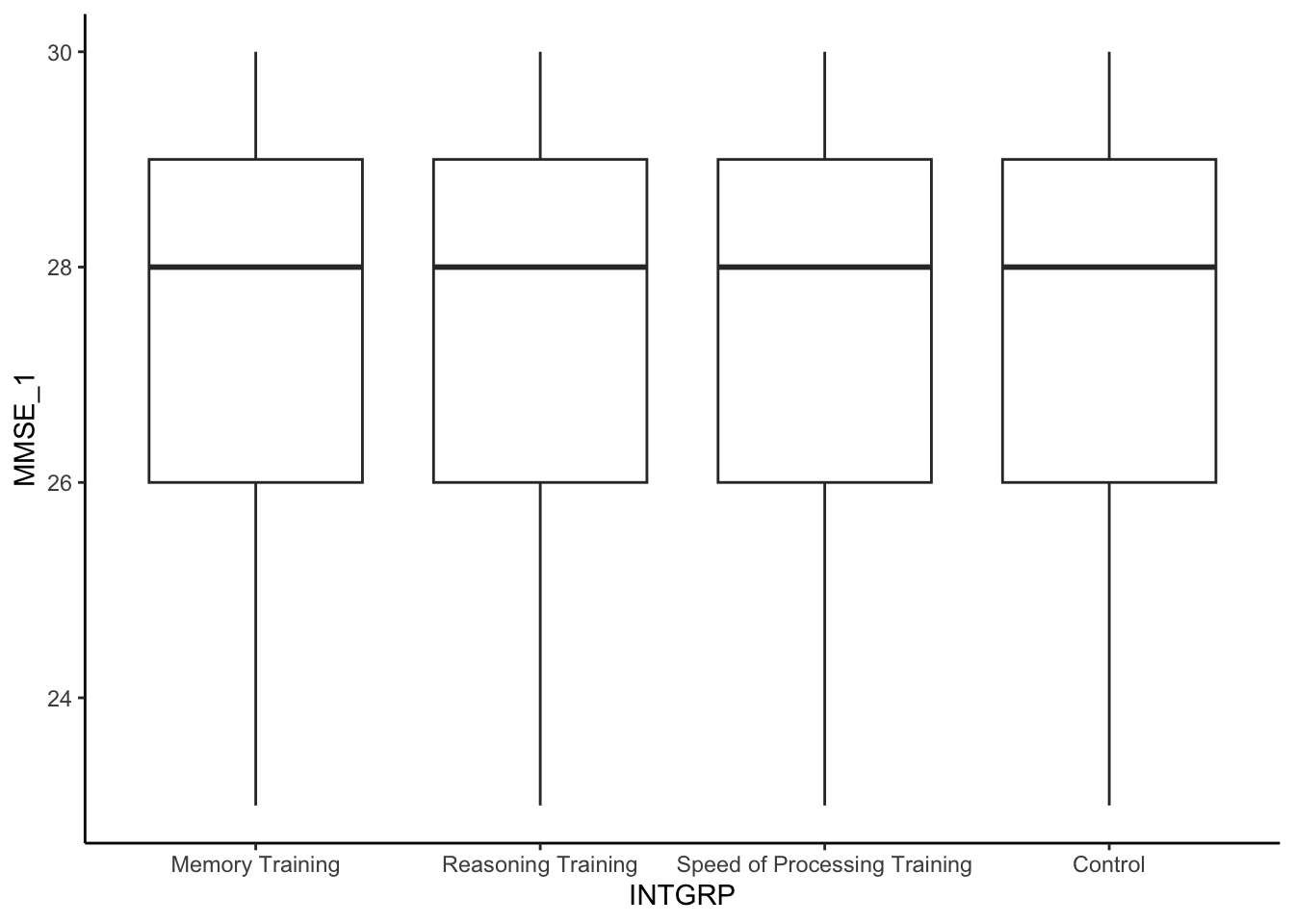
active %>%
  ggplot(aes(fill = INTGRP, x = MMSE_1)) +
  geom_density(alpha=0.2) +
  theme_classic()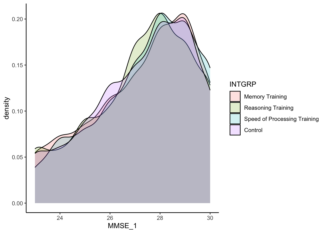
- .
Solution
There is a lot of variation in memory scores across the subjects and within subjects across time.
activeLong %>%
  ggplot(aes(x = Years, y = Memory, color = INTGRP, group = AID)) +
  geom_point(alpha = 0.2) +
  geom_line(alpha = 0.2) +
  theme_classic()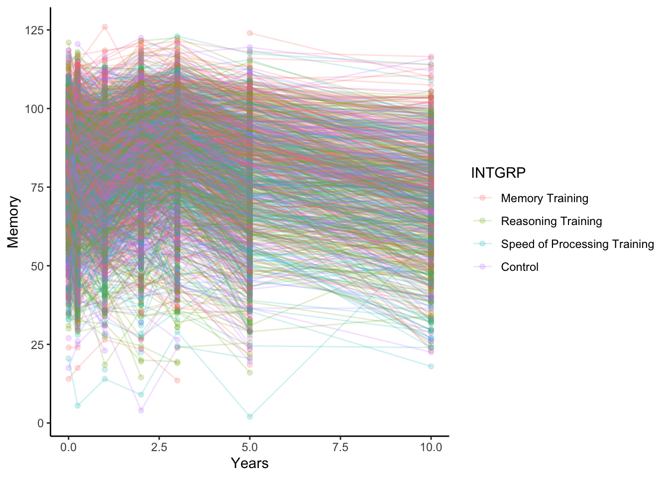
- .
Solution
On average, those in the memory training group performed better at all years of follow up. There was an increase in their memory score (across all groups) around years 2-3 but then a decline on average.
activeLong %>%
  group_by(INTGRP,Years) %>%
  summarize(Memory = mean(Memory, na.rm=TRUE)) %>%
  ggplot(aes(x = Years, y = Memory, color = INTGRP)) +
  geom_point() +
  geom_line() +
  labs(color = 'Treatment Group',y='Average Memory Score',x='Years of Follow Up') +
  theme_classic()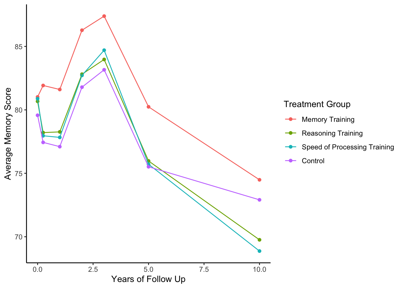
Discuss Models
- .
Solution
If you write Memory ~ Years + INTGRP, you are assuming a straight line relationships between Years and Memory and you are assuming that the relationships of Years and Memory is the same for each treatment group. With this model, treatment group shifts the intercept of the relationships.
If you write Memory ~ factor(Years) + INTGRP, you are now allowing a different mean Memory for each Year (allowing a non-linear relationship between Years and Memory) but you are assuming that the relationships of Years and Memory is the same for each treatment group. With this model, treatment group shifts the intercept of the relationships.
If you write Memory ~ factor(Years)*INTGRP, you are now allowing a different non-linear relationship between Memory and Year (allowing a non-linear relationship between Years and Memory) for each treatment group.
If you write Memory ~ bs(Years, knots=c(3), degree = 1)*INTGRP, you are allowing a linear piecewise relationships between Memory and Year and allow it to be different for each treatment group.
Solution
The estimates should be valid from lm() but we shouldn’t use the standard errors because we have repeated measurements over time on the same subjects.
Fit Models
- .
Solution
For either model you fit, you should notice that the model estimates a higher memory score on average for the Memory Training group over the Control group. With an interaction, we note that it is higher at baseline and impacts the relationship over time. We shouldn’t overly interpret the standard errors though to determine significance.
library(splines)
activeLong <- activeLong %>% mutate(INTGRP = relevel(INTGRP, ref='Control'))

activeLong %>% drop_na(Memory,Years,INTGRP) %>%
lm(Memory ~ factor(Years)*INTGRP, data = .) %>% summary()
Call:
lm(formula = Memory ~ factor(Years) * INTGRP, data = .)

Residuals:
    Min      1Q  Median      3Q     Max
-77.789 -10.777   1.564  12.578  45.129

Coefficients:
                                                     Estimate Std. Error
(Intercept)                                          79.57395    0.68857
factor(Years)0.25                                    -2.13746    0.97379
factor(Years)1                                       -2.47316    1.02808
factor(Years)2                                        2.21463    1.04767
factor(Years)3                                        3.58424    1.07481
factor(Years)5                                       -4.05765    1.12939
factor(Years)10                                      -6.66420    1.38301
INTGRPMemory Training                                 1.44459    0.97457
INTGRPReasoning Training                              1.09720    0.97031
INTGRPSpeed of Processing Training                    1.30605    0.97262
factor(Years)0.25:INTGRPMemory Training               3.04064    1.37660
factor(Years)1:INTGRPMemory Training                  3.06059    1.44943
factor(Years)2:INTGRPMemory Training                  3.04404    1.47236
factor(Years)3:INTGRPMemory Training                  2.78501    1.50777
factor(Years)5:INTGRPMemory Training                  3.27926    1.58909
factor(Years)10:INTGRPMemory Training                 0.13413    1.93582
factor(Years)0.25:INTGRPReasoning Training           -0.32557    1.37665
factor(Years)1:INTGRPReasoning Training               0.06683    1.45160
factor(Years)2:INTGRPReasoning Training              -0.07641    1.47627
factor(Years)3:INTGRPReasoning Training              -0.28252    1.50409
factor(Years)5:INTGRPReasoning Training              -0.63969    1.57427
factor(Years)10:INTGRPReasoning Training             -4.24862    1.89970
factor(Years)0.25:INTGRPSpeed of Processing Training -0.78401    1.37173
factor(Years)1:INTGRPSpeed of Processing Training    -0.57668    1.44624
factor(Years)2:INTGRPSpeed of Processing Training    -0.37556    1.47230
factor(Years)3:INTGRPSpeed of Processing Training     0.23837    1.50651
factor(Years)5:INTGRPSpeed of Processing Training    -1.10610    1.57628
factor(Years)10:INTGRPSpeed of Processing Training   -5.34456    1.91057
                                                     t value Pr(>|t|)
(Intercept)                                          115.564  < 2e-16 ***
factor(Years)0.25                                     -2.195 0.028181 *
factor(Years)1                                        -2.406 0.016159 *
factor(Years)2                                         2.114 0.034546 *
factor(Years)3                                         3.335 0.000856 ***
factor(Years)5                                        -3.593 0.000328 ***
factor(Years)10                                       -4.819 1.46e-06 ***
INTGRPMemory Training                                  1.482 0.138289
INTGRPReasoning Training                               1.131 0.258170
INTGRPSpeed of Processing Training                     1.343 0.179355
factor(Years)0.25:INTGRPMemory Training                2.209 0.027205 *
factor(Years)1:INTGRPMemory Training                   2.112 0.034741 *
factor(Years)2:INTGRPMemory Training                   2.067 0.038711 *
factor(Years)3:INTGRPMemory Training                   1.847 0.064755 .
factor(Years)5:INTGRPMemory Training                   2.064 0.039075 *
factor(Years)10:INTGRPMemory Training                  0.069 0.944761
factor(Years)0.25:INTGRPReasoning Training            -0.236 0.813054
factor(Years)1:INTGRPReasoning Training                0.046 0.963280
factor(Years)2:INTGRPReasoning Training               -0.052 0.958722
factor(Years)3:INTGRPReasoning Training               -0.188 0.851012
factor(Years)5:INTGRPReasoning Training               -0.406 0.684498
factor(Years)10:INTGRPReasoning Training              -2.236 0.025338 *
factor(Years)0.25:INTGRPSpeed of Processing Training  -0.572 0.567636
factor(Years)1:INTGRPSpeed of Processing Training     -0.399 0.690087
factor(Years)2:INTGRPSpeed of Processing Training     -0.255 0.798661
factor(Years)3:INTGRPSpeed of Processing Training      0.158 0.874280
factor(Years)5:INTGRPSpeed of Processing Training     -0.702 0.482868
factor(Years)10:INTGRPSpeed of Processing Training    -2.797 0.005160 **
---
Signif. codes:  0 '***' 0.001 '**' 0.01 '*' 0.05 '.' 0.1 ' ' 1

Residual standard error: 17.17 on 13226 degrees of freedom
Multiple R-squared:  0.04633,   Adjusted R-squared:  0.04438
F-statistic:  23.8 on 27 and 13226 DF,  p-value: < 2.2e-16
activeLong %>% drop_na(Memory,Years,INTGRP) %>%
lm(Memory ~ bs(Years,knots=c(3), degree = 1)*INTGRP, data = .) %>% summary()
Call:
lm(formula = Memory ~ bs(Years, knots = c(3), degree = 1) * INTGRP,
    data = .)

Residuals:
    Min      1Q  Median      3Q     Max
-76.467 -10.846   1.629  12.582  46.478

Coefficients:
                                                                        Estimate
(Intercept)                                                             78.02357
bs(Years, knots = c(3), degree = 1)1                                     3.44038
bs(Years, knots = c(3), degree = 1)2                                    -6.68111
INTGRPMemory Training                                                    3.04711
INTGRPReasoning Training                                                 0.99452
INTGRPSpeed of Processing Training                                       0.77678
bs(Years, knots = c(3), degree = 1)1:INTGRPMemory Training               2.05415
bs(Years, knots = c(3), degree = 1)2:INTGRPMemory Training              -1.16233
bs(Years, knots = c(3), degree = 1)1:INTGRPReasoning Training            0.08838
bs(Years, knots = c(3), degree = 1)2:INTGRPReasoning Training           -3.80495
bs(Years, knots = c(3), degree = 1)1:INTGRPSpeed of Processing Training  0.60504
bs(Years, knots = c(3), degree = 1)2:INTGRPSpeed of Processing Training -4.59747
                                                                        Std. Error
(Intercept)                                                                0.47087
bs(Years, knots = c(3), degree = 1)1                                       0.84892
bs(Years, knots = c(3), degree = 1)2                                       1.21681
INTGRPMemory Training                                                      0.66484
INTGRPReasoning Training                                                   0.66499
INTGRPSpeed of Processing Training                                         0.66269
bs(Years, knots = c(3), degree = 1)1:INTGRPMemory Training                 1.19128
bs(Years, knots = c(3), degree = 1)2:INTGRPMemory Training                 1.70059
bs(Years, knots = c(3), degree = 1)1:INTGRPReasoning Training              1.18874
bs(Years, knots = c(3), degree = 1)2:INTGRPReasoning Training              1.66848
bs(Years, knots = c(3), degree = 1)1:INTGRPSpeed of Processing Training    1.18775
bs(Years, knots = c(3), degree = 1)2:INTGRPSpeed of Processing Training    1.67625
                                                                        t value
(Intercept)                                                             165.700
bs(Years, knots = c(3), degree = 1)1                                      4.053
bs(Years, knots = c(3), degree = 1)2                                     -5.491
INTGRPMemory Training                                                     4.583
INTGRPReasoning Training                                                  1.496
INTGRPSpeed of Processing Training                                        1.172
bs(Years, knots = c(3), degree = 1)1:INTGRPMemory Training                1.724
bs(Years, knots = c(3), degree = 1)2:INTGRPMemory Training               -0.683
bs(Years, knots = c(3), degree = 1)1:INTGRPReasoning Training             0.074
bs(Years, knots = c(3), degree = 1)2:INTGRPReasoning Training            -2.280
bs(Years, knots = c(3), degree = 1)1:INTGRPSpeed of Processing Training   0.509
bs(Years, knots = c(3), degree = 1)2:INTGRPSpeed of Processing Training  -2.743
                                                                        Pr(>|t|)
(Intercept)                                                              < 2e-16
bs(Years, knots = c(3), degree = 1)1                                    5.09e-05
bs(Years, knots = c(3), degree = 1)2                                    4.08e-08
INTGRPMemory Training                                                   4.62e-06
INTGRPReasoning Training                                                  0.1348
INTGRPSpeed of Processing Training                                        0.2412
bs(Years, knots = c(3), degree = 1)1:INTGRPMemory Training                0.0847
bs(Years, knots = c(3), degree = 1)2:INTGRPMemory Training                0.4943
bs(Years, knots = c(3), degree = 1)1:INTGRPReasoning Training             0.9407
bs(Years, knots = c(3), degree = 1)2:INTGRPReasoning Training             0.0226
bs(Years, knots = c(3), degree = 1)1:INTGRPSpeed of Processing Training   0.6105
bs(Years, knots = c(3), degree = 1)2:INTGRPSpeed of Processing Training   0.0061

(Intercept)                                                             ***
bs(Years, knots = c(3), degree = 1)1                                    ***
bs(Years, knots = c(3), degree = 1)2                                    ***
INTGRPMemory Training                                                   ***
INTGRPReasoning Training
INTGRPSpeed of Processing Training
bs(Years, knots = c(3), degree = 1)1:INTGRPMemory Training              .
bs(Years, knots = c(3), degree = 1)2:INTGRPMemory Training
bs(Years, knots = c(3), degree = 1)1:INTGRPReasoning Training
bs(Years, knots = c(3), degree = 1)2:INTGRPReasoning Training           *
bs(Years, knots = c(3), degree = 1)1:INTGRPSpeed of Processing Training
bs(Years, knots = c(3), degree = 1)2:INTGRPSpeed of Processing Training **
---
Signif. codes:  0 '***' 0.001 '**' 0.01 '*' 0.05 '.' 0.1 ' ' 1

Residual standard error: 17.24 on 13242 degrees of freedom
Multiple R-squared:  0.03728,   Adjusted R-squared:  0.03648
F-statistic: 46.61 on 11 and 13242 DF, p-value: < 2.2e-16- .
Solution
The Model SE is the same as lm(). For this data set, the Robust SE are smaller than the Std. Error from lm(), which is counterintuitive because we’d expect that we don’t have as much unique information as the full sample size would indicate since we have correlated observations. We’d expect higher uncertainty and more variability with smaller effective sample sizes.
library(geeM)
library(tidyr)

activeLong %>% drop_na(Memory,Years,INTGRP) %>%
  geem(Memory ~ factor(Years)*INTGRP, data = ., id = AID, corstr = 'independence') %>% #independent working correlation
  summary()
Estimates Model SE
(Intercept) 79.57000 0.6886
factor(Years)0.25 -2.13700 0.9738
factor(Years)1 -2.47300 1.0280
factor(Years)2 2.21500 1.0480
factor(Years)3 3.58400 1.0750
factor(Years)5 -4.05800 1.1290
factor(Years)10 -6.66400 1.3830
INTGRPMemory Training 1.44500 0.9746
INTGRPReasoning Training 1.09700 0.9703
INTGRPSpeed of Processing Training 1.30600 0.9726
factor(Years)0.25:INTGRPMemory Training 3.04100 1.3770
factor(Years)1:INTGRPMemory Training 3.06100 1.4490
factor(Years)2:INTGRPMemory Training 3.04400 1.4720
factor(Years)3:INTGRPMemory Training 2.78500 1.5080
factor(Years)5:INTGRPMemory Training 3.27900 1.5890
factor(Years)10:INTGRPMemory Training 0.13410 1.9360
factor(Years)0.25:INTGRPReasoning Training -0.32560 1.3770
factor(Years)1:INTGRPReasoning Training 0.06683 1.4520
factor(Years)2:INTGRPReasoning Training -0.07641 1.4760
factor(Years)3:INTGRPReasoning Training -0.28250 1.5040
factor(Years)5:INTGRPReasoning Training -0.63970 1.5740
factor(Years)10:INTGRPReasoning Training -4.24900 1.9000
factor(Years)0.25:INTGRPSpeed of Processing Training -0.78400 1.3720
factor(Years)1:INTGRPSpeed of Processing Training -0.57670 1.4460
factor(Years)2:INTGRPSpeed of Processing Training -0.37560 1.4720
factor(Years)3:INTGRPSpeed of Processing Training 0.23840 1.5070
factor(Years)5:INTGRPSpeed of Processing Training -1.10600 1.5760
factor(Years)10:INTGRPSpeed of Processing Training -5.34500 1.9110
Robust SE wald
(Intercept) 0.6656 119.60000
factor(Years)0.25 0.5079 -4.20800
factor(Years)1 0.5889 -4.20000
factor(Years)2 0.6902 3.20900
factor(Years)3 0.7094 5.05300
factor(Years)5 0.9038 -4.48900
factor(Years)10 1.2230 -5.45100
INTGRPMemory Training 0.9293 1.55400
INTGRPReasoning Training 0.9107 1.20500
INTGRPSpeed of Processing Training 0.9195 1.42000
factor(Years)0.25:INTGRPMemory Training 0.7225 4.20900
factor(Years)1:INTGRPMemory Training 0.8300 3.68700
factor(Years)2:INTGRPMemory Training 0.9408 3.23600
factor(Years)3:INTGRPMemory Training 0.9905 2.81200
factor(Years)5:INTGRPMemory Training 1.2740 2.57400
factor(Years)10:INTGRPMemory Training 1.7520 0.07655
factor(Years)0.25:INTGRPReasoning Training 0.7073 -0.46030
factor(Years)1:INTGRPReasoning Training 0.8188 0.08162
factor(Years)2:INTGRPReasoning Training 0.9476 -0.08064
factor(Years)3:INTGRPReasoning Training 0.9723 -0.29060
factor(Years)5:INTGRPReasoning Training 1.2090 -0.52910
factor(Years)10:INTGRPReasoning Training 1.6000 -2.65500
factor(Years)0.25:INTGRPSpeed of Processing Training 0.6761 -1.16000
factor(Years)1:INTGRPSpeed of Processing Training 0.8108 -0.71130
factor(Years)2:INTGRPSpeed of Processing Training 0.9274 -0.40500
factor(Years)3:INTGRPSpeed of Processing Training 0.9479 0.25150
factor(Years)5:INTGRPSpeed of Processing Training 1.1840 -0.93390
factor(Years)10:INTGRPSpeed of Processing Training 1.6880 -3.16600
p
(Intercept) 0.000e+00
factor(Years)0.25 2.572e-05
factor(Years)1 2.670e-05
factor(Years)2 1.334e-03
factor(Years)3 4.400e-07
factor(Years)5 7.150e-06
factor(Years)10 5.000e-08
INTGRPMemory Training 1.201e-01
INTGRPReasoning Training 2.283e-01
INTGRPSpeed of Processing Training 1.555e-01
factor(Years)0.25:INTGRPMemory Training 2.570e-05
factor(Years)1:INTGRPMemory Training 2.266e-04
factor(Years)2:INTGRPMemory Training 1.214e-03
factor(Years)3:INTGRPMemory Training 4.927e-03
factor(Years)5:INTGRPMemory Training 1.006e-02
factor(Years)10:INTGRPMemory Training 9.390e-01
factor(Years)0.25:INTGRPReasoning Training 6.453e-01
factor(Years)1:INTGRPReasoning Training 9.350e-01
factor(Years)2:INTGRPReasoning Training 9.357e-01
factor(Years)3:INTGRPReasoning Training 7.714e-01
factor(Years)5:INTGRPReasoning Training 5.968e-01
factor(Years)10:INTGRPReasoning Training 7.930e-03
factor(Years)0.25:INTGRPSpeed of Processing Training 2.462e-01
factor(Years)1:INTGRPSpeed of Processing Training 4.769e-01
factor(Years)2:INTGRPSpeed of Processing Training 6.855e-01
factor(Years)3:INTGRPSpeed of Processing Training 8.014e-01
factor(Years)5:INTGRPSpeed of Processing Training 3.504e-01
factor(Years)10:INTGRPSpeed of Processing Training 1.545e-03
Estimated Correlation Parameter: 0
Correlation Structure: independence
Est. Scale Parameter: 294.9
Number of GEE iterations: 2
Number of Clusters: 2785 Maximum Cluster Size: 7
Number of observations with nonzero weight: 13254 - .
Solution
The Model SE and Robust SE are much closer together for this model (ar1 working correlation structure) than when we used the independence working correlation structure. This indicates that this model for correlation is more closer to the truth than the independence working correlation structure.
activeLong %>% drop_na(Memory,Years,INTGRP) %>%
  geem(Memory ~ factor(Years)*INTGRP, data = ., id = AID, corstr = 'ar1') %>% #ar1 working correlation
  summary()
Estimates Model SE
(Intercept) 79.89000 0.6666
factor(Years)0.25 -2.80700 0.4403
factor(Years)1 -4.36700 0.5973
factor(Years)2 -0.07463 0.6928
factor(Years)3 1.25900 0.7733
factor(Years)5 -7.99200 0.8600
factor(Years)10 -14.20000 0.7296
INTGRPMemory Training 1.50300 0.9416
INTGRPReasoning Training 1.09300 0.9406
INTGRPSpeed of Processing Training 1.18600 0.9410
factor(Years)0.25:INTGRPMemory Training 2.85300 0.6239
factor(Years)1:INTGRPMemory Training 2.65000 0.8426
factor(Years)2:INTGRPMemory Training 2.93400 0.9738
factor(Years)3:INTGRPMemory Training 2.54400 1.0850
factor(Years)5:INTGRPMemory Training 3.50000 1.2090
factor(Years)10:INTGRPMemory Training 0.39270 1.0180
factor(Years)0.25:INTGRPReasoning Training 0.00136 0.6232
factor(Years)1:INTGRPReasoning Training 0.28040 0.8443
factor(Years)2:INTGRPReasoning Training 0.05498 0.9772
factor(Years)3:INTGRPReasoning Training -0.27730 1.0860
factor(Years)5:INTGRPReasoning Training 0.34430 1.2060
factor(Years)10:INTGRPReasoning Training -2.18600 0.9945
factor(Years)0.25:INTGRPSpeed of Processing Training 0.08228 0.6193
factor(Years)1:INTGRPSpeed of Processing Training 0.18980 0.8390
factor(Years)2:INTGRPSpeed of Processing Training -0.05613 0.9718
factor(Years)3:INTGRPSpeed of Processing Training 0.36120 1.0820
factor(Years)5:INTGRPSpeed of Processing Training 0.46470 1.1980
factor(Years)10:INTGRPSpeed of Processing Training -1.55200 1.0010
Robust SE wald
(Intercept) 0.6489 123.100000
factor(Years)0.25 0.3945 -7.116000
factor(Years)1 0.4581 -9.532000
factor(Years)2 0.5361 -0.139200
factor(Years)3 0.5373 2.344000
factor(Years)5 0.7153 -11.170000
factor(Years)10 0.9406 -15.100000
INTGRPMemory Training 0.9035 1.663000
INTGRPReasoning Training 0.8883 1.231000
INTGRPSpeed of Processing Training 0.8923 1.330000
factor(Years)0.25:INTGRPMemory Training 0.5534 5.155000
factor(Years)1:INTGRPMemory Training 0.6246 4.242000
factor(Years)2:INTGRPMemory Training 0.7104 4.130000
factor(Years)3:INTGRPMemory Training 0.7490 3.397000
factor(Years)5:INTGRPMemory Training 0.9900 3.536000
factor(Years)10:INTGRPMemory Training 1.3320 0.294700
factor(Years)0.25:INTGRPReasoning Training 0.5592 0.002432
factor(Years)1:INTGRPReasoning Training 0.6194 0.452600
factor(Years)2:INTGRPReasoning Training 0.7303 0.075280
factor(Years)3:INTGRPReasoning Training 0.7319 -0.378800
factor(Years)5:INTGRPReasoning Training 0.9495 0.362600
factor(Years)10:INTGRPReasoning Training 1.2280 -1.780000
factor(Years)0.25:INTGRPSpeed of Processing Training 0.5520 0.149100
factor(Years)1:INTGRPSpeed of Processing Training 0.6284 0.302100
factor(Years)2:INTGRPSpeed of Processing Training 0.7225 -0.077690
factor(Years)3:INTGRPSpeed of Processing Training 0.7253 0.498000
factor(Years)5:INTGRPSpeed of Processing Training 0.9307 0.499300
factor(Years)10:INTGRPSpeed of Processing Training 1.3240 -1.173000
p
(Intercept) 0.000e+00
factor(Years)0.25 0.000e+00
factor(Years)1 0.000e+00
factor(Years)2 8.893e-01
factor(Years)3 1.908e-02
factor(Years)5 0.000e+00
factor(Years)10 0.000e+00
INTGRPMemory Training 9.622e-02
INTGRPReasoning Training 2.183e-01
INTGRPSpeed of Processing Training 1.837e-01
factor(Years)0.25:INTGRPMemory Training 2.500e-07
factor(Years)1:INTGRPMemory Training 2.213e-05
factor(Years)2:INTGRPMemory Training 3.631e-05
factor(Years)3:INTGRPMemory Training 6.818e-04
factor(Years)5:INTGRPMemory Training 4.069e-04
factor(Years)10:INTGRPMemory Training 7.682e-01
factor(Years)0.25:INTGRPReasoning Training 9.981e-01
factor(Years)1:INTGRPReasoning Training 6.508e-01
factor(Years)2:INTGRPReasoning Training 9.400e-01
factor(Years)3:INTGRPReasoning Training 7.048e-01
factor(Years)5:INTGRPReasoning Training 7.169e-01
factor(Years)10:INTGRPReasoning Training 7.513e-02
factor(Years)0.25:INTGRPSpeed of Processing Training 8.815e-01
factor(Years)1:INTGRPSpeed of Processing Training 7.626e-01
factor(Years)2:INTGRPSpeed of Processing Training 9.381e-01
factor(Years)3:INTGRPSpeed of Processing Training 6.185e-01
factor(Years)5:INTGRPSpeed of Processing Training 6.175e-01
factor(Years)10:INTGRPSpeed of Processing Training 2.409e-01
Estimated Correlation Parameter: 0.8066
Correlation Structure: ar1
Est. Scale Parameter: 299.7
Number of GEE iterations: 5
Number of Clusters: 2785 Maximum Cluster Size: 7
Number of observations with nonzero weight: 13254 - .
Solution
Based on this model above, we can see that at baseline (Years = 0), there is not a discernible difference in mean memory score between treatment groups (which is good!!) [Looking at estimates and p-values for INTGRPMemory Training, INTGRPReasoning Training, and INTGRPSpeed of Processing Training].
We can also see that there is a discernible difference in the Year = 0 to Year = 2 increase for Memory Training as compared to the Control group [looking at estimates of factor(Years)2:INTGRPMemory Training] but there aren’t discernible differences in mean memory in the Year = 0 to Year = 10 change for Memory Training as compared to Control group [looking at estimates of factor(Years)10:INTGRPMemory Training]. There aren’t discernible differences between the other training groups and the control group across time. So maybe there isn’t that much of a difference or relationship between the Memory training? It is worth pursuing further.Wrap-Up
Finishing the Activity
- If you didn’t finish the activity, no problem! Be sure to complete the activity outside of class, review the solutions in the online manual, and ask any questions on Slack or in office hours.
- Re-organize and review your notes to help deepen your understanding, solidify your learning, and make homework go more smoothly!
After Class
Before the next class, please do the following:
- Take a look at the Schedule page to see how to prepare for the next class.