astsa::acf2(y)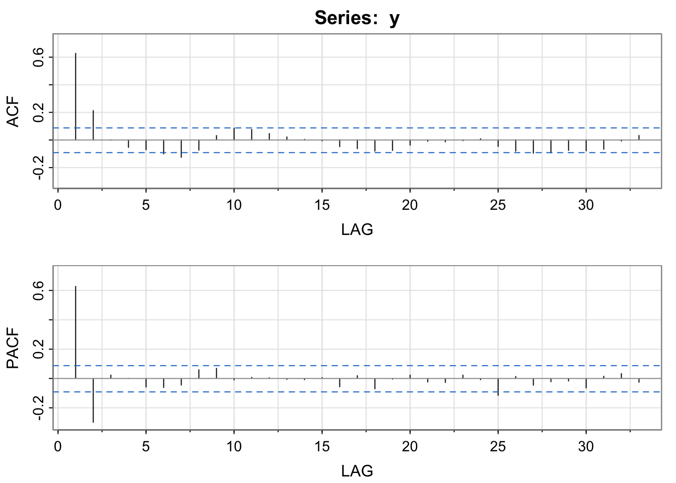
Once you’ve removed trend and seasonality,
sarima(data, p, d, q)sarima() - want high p-values for Ljung-Box and ACF that looks like independent noise. . .
Example
astsa::acf2(y)
Candidate List: AR(1), AR(2), MA(2)
# Fit all models - Check out Diagnostic plots
mod_ar1 <- sarima(y, p = 1, d = 0, q = 0)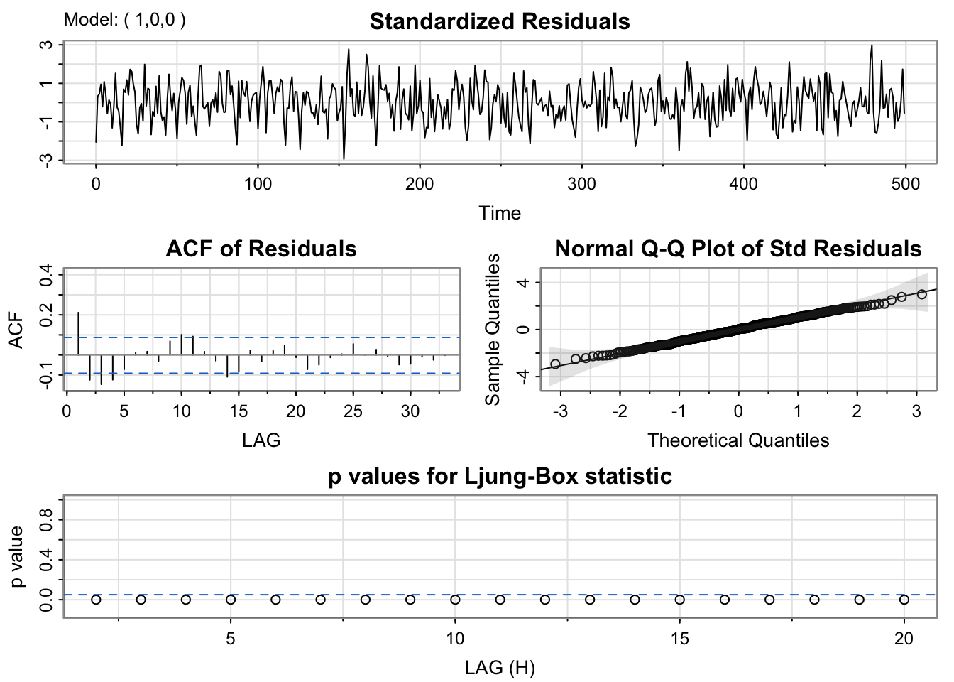
mod_ar2 <- sarima(y, p = 2, d = 0, q = 0)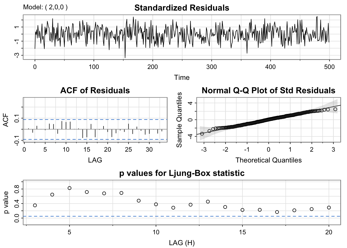
mod_ma2 <- sarima(y, p = 0, d = 0, q = 2)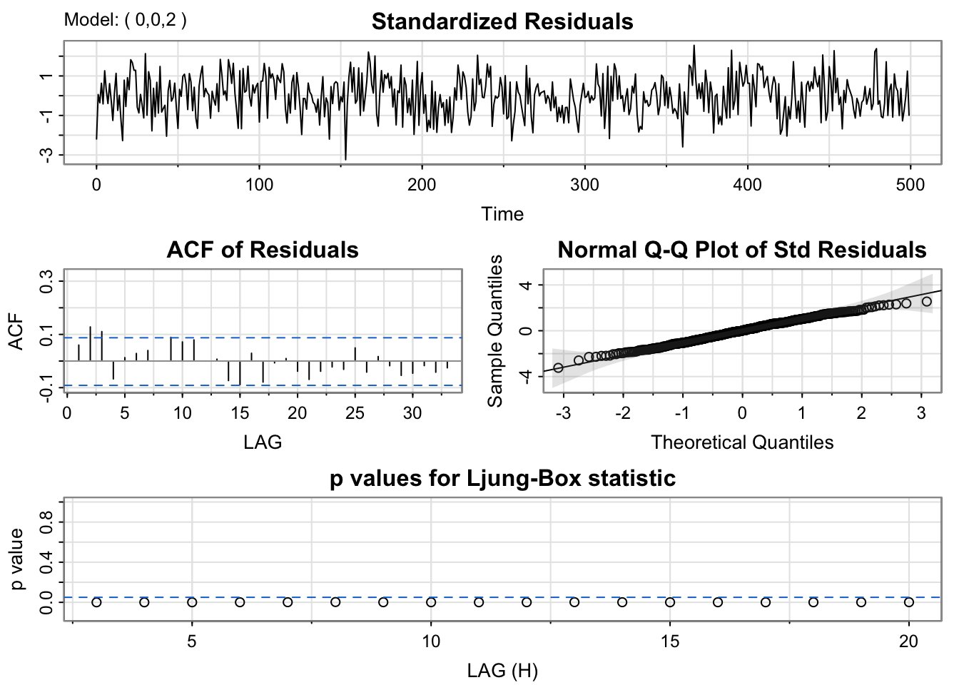
# Check H0: phi = 0
mod_ar1$ttable
Estimate SE t.value p.value
ar1 0.7208 0.0311 23.1857 0.0000
xmean 0.0540 0.1754 0.3080 0.7582mod_ar2$ttable Estimate SE t.value p.value
ar1 0.9378 0.0427 21.9670 0.0000
ar2 -0.3022 0.0428 -7.0666 0.0000
xmean 0.0608 0.1286 0.4728 0.6366mod_ma2$ttable Estimate SE t.value p.value
ma1 0.8966 0.0399 22.4968 0.0000
ma2 0.3722 0.0374 9.9620 0.0000
xmean 0.0630 0.1084 0.5817 0.5611# Check BIC, AIC (lower is better)
mod_ar1$ICs AIC AICc BIC
3.043172 3.043220 3.068459 mod_ar2$ICs AIC AICc BIC
2.952012 2.952109 2.985729 mod_ma2$ICs AIC AICc BIC
2.990376 2.990473 3.024093 
Incorporate Trend and Seasonality into the Model
Parametric Model: If we estimate the trend and seasonality using lm() [e.g. polynomials, splines, indicator variables, sine/cosine curves]
sarima(xreg = X) where X <- model.matrix(lm(y ~ x, data )) .. . .
But what does model.matrix() do? or
model.matrix(lm(y ~ x, data)) or model.matrix(~ x, data)
. . .
Differencing:
If we use differencing to remove trend and seasonality,
sarima(d, D, S) where d is the order of lag = 1 differences to remove trend, D is the order of lag = S differences to remove seasonality.But why do we need one final model?
. . .
Simultaneous Estimation of All Components
Once we’ve made choices for each model component, it is useful to simultaneously estimate one final model
BUT, what if the residuals from your Noise Model don’t look like independent noise?
It can be useful to use the backshift operator, \(B\), to simplify the notation of our models, such that
\[B^k Y_t = Y_{t-k}\text{ for }k = 0,1,2,3,4,...\]
Our \(AR(p)\) can be written as
\[(1 - \phi_1B - \cdots-\phi_pB^p)Y_t = W_t\]
Our \(MA(q)\) can be written as
\[Y_t = (1 + \theta_1B + \cdots+\theta_qB^q)W_t\]
. . .
We can use the backshift operator to simplify the notation for differences.
\[Y_t - Y_{t-1} = (1-B)Y_t\]
\[(Y_t - Y_{t-1}) - (Y_{t-1} - Y_{t-2}) = (1-B)^2Y_t\]
\[Y_t - Y_{t-S} = (1-B^S)Y_t\]
\[(1-B)(1-B^S)Y_t = (1 - B - B^{S} + B^{S+1}) Y_t = (Y_t - Y_{t-1}) - ( Y_{t-S}-Y_{t-S-1}) \]
Why a new model?
If you have removed seasonality (as best as you can) and fit the best possible ARMA model you can…
But if you see a strong seasonal pattern in the residuals (after the ARMA Model),
SOLUTION: You could try to incorporate a Seasonal AR or MA component.
S, 2S, 3S, etc.. . .
Definitions:
A Seasonal \(AR(P)\) can be written as
\[(1 - \Phi_1B^S - \cdots-\Phi_PB^{PS})Y_t = W_t\]
A Seasonal \(MA(Q)\) can be written as
\[Y_t = (1 + \Theta_1B^S + \cdots+\Theta_QB^{QS})W_t\]
All together, an \(ARMA(p,q)\) + Seasonal \(ARMA(P,Q)\)
\[(1 - \Phi_1B^S - \cdots-\Phi_PB^{PS})(1 - \phi_1B - \cdots-\phi_pB^p)Y_t \] \[ = (1 + \Theta_1B^S + \cdots+\Theta_QB^{QS})(1 + \theta_1B + \cdots+\theta_qB^q)W_t\]
. . .
Seasonal ARMA Model Selection
To determine the order of a seasonal ARMA, look for patterns on \(j*S\) lags.
Seasonal \(AR(P)\):
S, 2S, 3S,...;PS along lags S, 2S, 3S, ...Seasonal \(MA(Q)\):
QS along lags S, 2S, 3S,...;S, 2S, 3S,.... . .
Implementation
To fit a SARIMA model, add order P and Q into the \(ARMA(p,q)\) model with
sarima(p,d,q,P,D,Q,S)Forecasting is one form of extrapolating to make predictions for the future (unobserved values of the random process).
To forecast, we need to consider predicting the trend, seasonality, and the noise
\[\hat{y}_{t+1} = \underbrace{\hat{f}(t+1|y_1,...,y_{t})}_{trend} + \underbrace{\hat{S}(t+1|y_1,...,y_t)}_{seasonality} + \underbrace{\hat{e}_{t+1}}_{noise}\]
There is no one “best” way to forecast the trend of a time series.
Some Approaches
. . .
What assumptions do you make for each of these approaches?
There is no one “best” way to forecast the trend of a time series.
Some Approaches
Seasonal Naive: Predicted seasonality = last observed value from same season
Seasonal Curve: Predicted seasonality = predicted value from a linear model [with indicator variables or sine/cosine curves]
. . .
What assumptions do you make for each of these approaches?
Some Approaches
Naive: If noise has mean 0, predict noise is 0.
ARMA Model: Prediction = predicted value using parameter estimates, observed data and residuals
ARIMA: Prediction = predicted value using parameter estimates, observed data and their differences
Implementation
In R: we can use our one final model to forecast into the future using the astsa::sarima.for() function.
astsa::sarima.for(orig_data, p, d, q, P, D, Q, S, xreg, newxreg, n.ahead)xreg, newxregn.aheadNote:
newxreg, you must create a variable with dates in future.newdat <- data.frame(date = max(data$date) %m+% months(1:24)) %>% # extend out 24 months
mutate(dec_date = decimal_date(date), month = month(date)) # create date/time variables used in modelsmodel.matrix to create a matrix used in model formula to pass to sarima.for.NewX <- model.matrix(formula, data = newdat)[, -1] # -1 removes intercept columnformula <- y ~ bs(dec_date, Boundary.knots = c(min(dec_date), max(dec_date) + n.ahead/12 ) #example for monthly dataDownload a template Qmd file to start from here.
Below, there is three R code chunks to generate three time series and show the theoretical and estimated ACF.
sarima.sarima.for.Model 1:
\[Y_t = \]
library(dplyr)
library(astsa)

y1 <- sarima.sim(ar = c(0.9, -0.1))
plot(y1, type='l')

#estimated ACF and PACF
acf2(y1)

#theoretical ACF and PACF
ARMAacf(ar = c(0.9, -0.1),lag.max = 20) %>% plot(type='h',ylim=c(-1,1))

ARMAacf(ar = c(0.9, -0.1), pacf = TRUE,lag.max = 20) %>% plot(type='h',ylim=c(-1,1))

#fit model to data


#forecast
Model 2:
\[Y_t = \]
y2 <- sarima.sim(ma = c(0.7), d = 1, D = 1, S = 6)
plot(y2, type='l')

#estimated ACF and PACF
y2 %>% diff(lag = 1) %>% diff(lag = 6) %>% acf2()

#theoretical ACF and PACF
ARMAacf(ma = 0.7, lag.max = 20) %>% plot(type='h',ylim=c(-1,1))
ARMAacf(ma = 0.7, pacf=TRUE,lag.max = 20) %>% plot(type='h',ylim=c(-1,1))

#fit model to data


#forecast
Model 3:
\[Y_t = \]
y3 <- sarima.sim(ar = c(0.9), sar = 0.5, S = 12)
plot(y3, type='l')

#estimated ACF and PACF
acf2(y3)

#theoretical ACF and PACF
ARMAacf(ar = c(0.9, rep(0, 10), 0.5, -0.9*0.5)) %>% plot(type='h',ylim=c(-1,1))

ARMAacf(ar = c(0.9, rep(0, 10), 0.5, -0.9*0.5), pacf=TRUE) %>% plot(type='h',ylim=c(-1,1))

#fit model to data


#forecast
Summarize your new understanding of SARIMA models and how the SARIMA is different/similar to ARMA models.
Model 1
AR(2)
\[Y_t = \phi_1Y_{t-1} +\phi_2 Y_{t-2} + W_t\] \[(1 - \phi_1B - \phi_2B^2)Y_t = W_t\]
library(dplyr)
library(astsa)

y1 <- sarima.sim(ar = c(0.9, -0.1))
plot(y1, type='l')

#estimated ACF and PACF
acf2(y1)

#theoretical ACF and PACF
ARMAacf(ar = c(0.9, -0.1),lag.max = 20) %>% plot(type='h',ylim=c(-1,1))
ARMAacf(ar = c(0.9, -0.1), pacf=TRUE,lag.max = 20) %>% plot(type='h',ylim=c(-1,1))

#fit model to data
fit.mod1 <- sarima(y1,p = 2,d = 0, q = 0)
fit.mod1

#forecast
sarima.for(y1,p = 2,d = 0, q = 0, n.ahead = 6 )
Model 2
MA(1) + Differencing
\[(1-B^6)(1-B)Y_t = (1 +\theta_1B) W_t\]
\[(1-B^6 - B+B^7)Y_t = (1 +\theta_1B) W_t\]
y2 <- sarima.sim(ma = c(0.7), d = 1, D = 1, S = 6)
plot(y2, type='l')

#estimated ACF and PACF
y2 %>% diff(lag = 1) %>% diff(lag = 6) %>% acf2()

#theoretical ACF and PACF
ARMAacf(ma = 0.7, lag.max = 20) %>% plot(type='h',ylim=c(-1,1))
ARMAacf(ma = 0.7, pacf=TRUE,lag.max = 20) %>% plot(type='h',ylim=c(-1,1))

#fit model to data
fit.mod2 <- sarima(y2, p = 0, d = 1, q = 1, D = 1, S = 6)
fit.mod2

#forecast
sarima.for(y2, p = 0, d = 1, q = 1, D = 1, S = 6, n.ahead = 6 )
Model 3
AR(1) + Seasonal AR(1)
\[(1-\Phi_1B^{12})(1-\phi_1B)Y_t = W_t\]
\[(1-\Phi_1B^{12} - \phi_1B+\phi_1\Phi_1B^{13})Y_t = W_t\]
y3 <- sarima.sim(ar = c(0.9), sar = 0.5, S = 12)
plot(y3, type='l')

#estimated ACF and PACF
acf2(y3)

#theoretical ACF and PACF
ARMAacf(ar = c(0.9, rep(0, 10), 0.5, -0.9*0.5)) %>% plot(type='h',ylim=c(-1,1))
ARMAacf(ar = c(0.9, rep(0, 10), 0.5, -0.9*0.5), pacf=TRUE) %>% plot(type='h',ylim=c(-1,1))

#fit model to data
fit.mod3 <- sarima(y3, p = 1, d = 0, q = 0, P = 1, D = 0, S = 12)
fit.mod3

#forecast
sarima.for(y3, p = 1, d = 0, q = 0, P = 1, D = 0, S = 12, n.ahead = 6 )Before the next class, please do the following: