Instead of: “We chose this covariance model because the BIC is 1200.”
Do this: “We chose this autoregressive order 1 covariance model because it has the same goodness of fit, as measured by BIC, as the more complex model. This suggests that there is covariance decays to zero as the time between observations increase, after accounting for the variation in the mean.”
. . .
Focus on the big picture conclusion
Use numeric values sparingly; only when it highly strengthens the argument.
Instead of: “The coefficients for Years are 0.5, 0.8, 0.9 , 0.7, and -0.5.”
Do this: “The model suggests that the average score increases for 3 years and then starts to decline, ending at a lower point than at baseline, after accounting for age and memory score at baseline.”
Mini Project 2
Due: Thursday in class
. . .
Audience: Stat 155 Students
Professional visualizations: make sure all of the “ink” in the graph is informative
. . .
What to Include:
An introduction to the ACTIVE study with parenthetical citations of relevant papers using Bibtex
An introduction to your research question and why it is important
An introduction to the data without using variable_names
A discussion and justification of your model (gee v. mixed effects; mean model; covariance model) that explains WHY you made your choices
A discussion of your conclusions based on the model and the limitations to the conclusions you can make.
Learning Goals
Explain and detect three different types of spatial data (point-referenced, point process, areal data)
Formulate research questions for the three types of spatial data
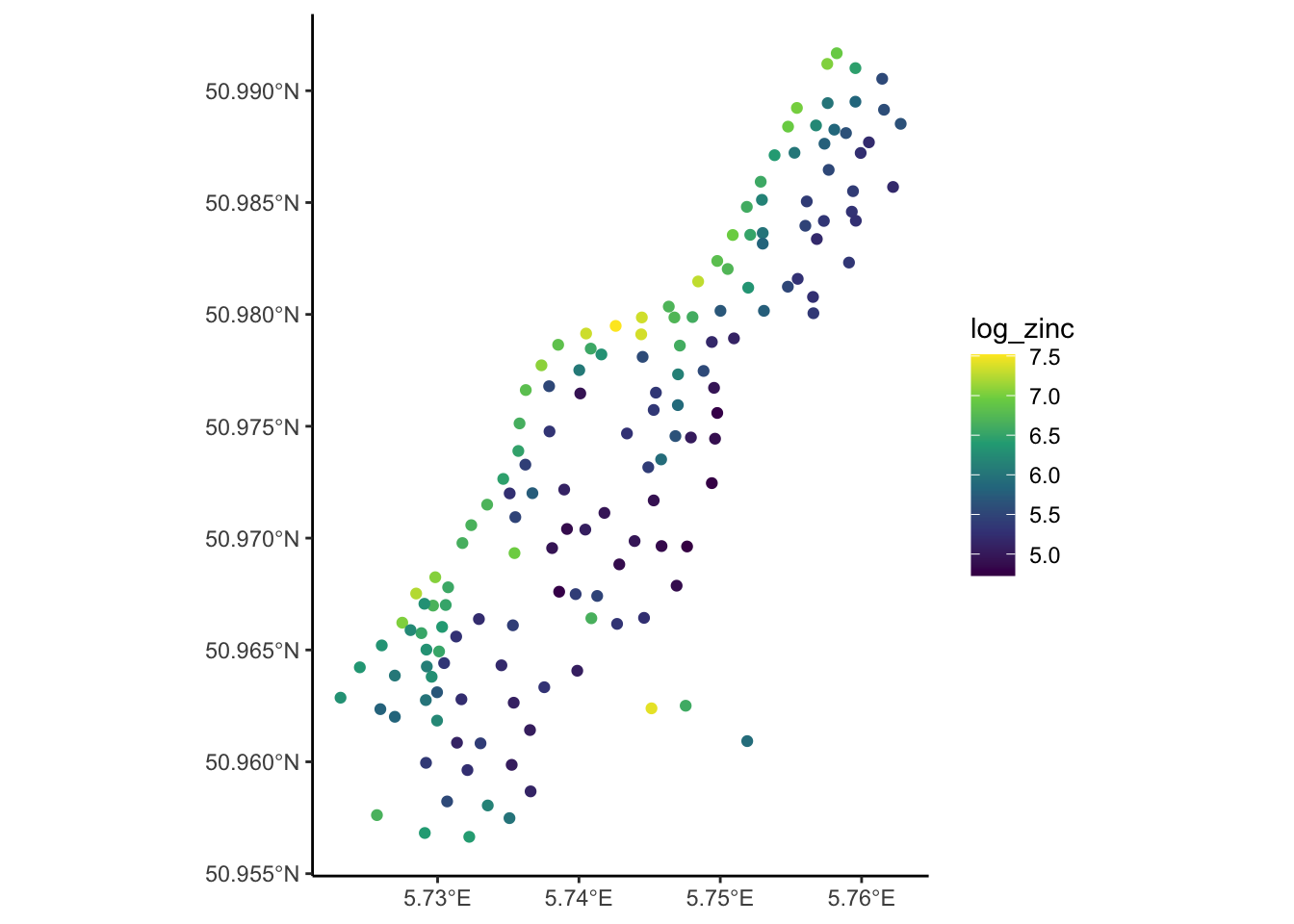
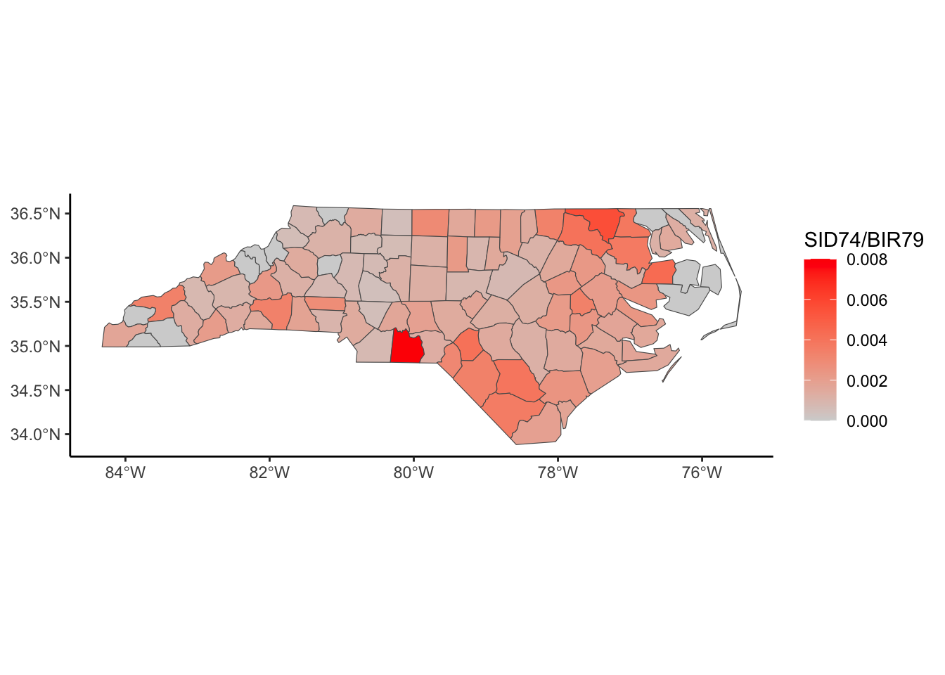
Point-Referenced (Geostatistical) Data
Geostatistical Research Questions
Can we explain the variation in an outcome variable Y that is measured in space?
Agriculture: Why do we get higher yield of a crop in one location versus another?
Geology: Why do we have higher metal concentrations in the soil in one location versus another?
Weather: Why do we have higher wind in one location versus another?
Environmental: Why do we have higher pollution in one location versus another?
. . .
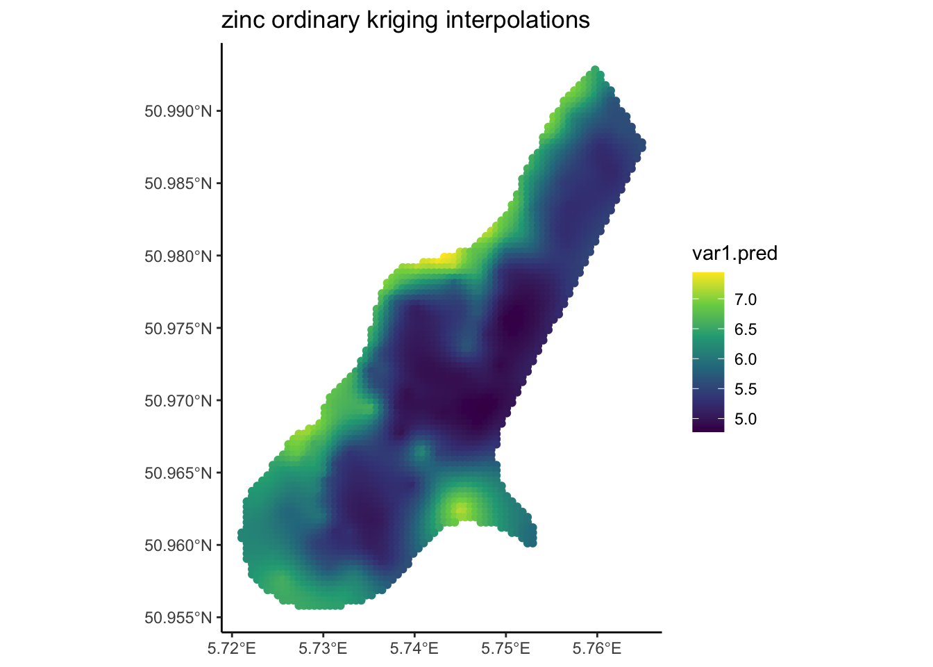
Can we predict an outcome variable Y at any spatial location given a smaller sample of data at spatial locations?
Agriculture: Predict yield for entire farm based on 50 samples.
Geology: Predict metal concentrations in the soil for a large area based on 100 samples.
Weather: Predict the weather at every location based on model estimates at a grid of locations.
Environmental: Prediction pollution levels at every location based on measurements at monitoring stations.
Geostatistical Data Structure
For a set of \(n\) spatial locations,
An outcome measurement Y,
Measurements of a variety of explanatory variables, X’s (e.g. elevation, distance to a location)
. . .
In order to do predictions,
You need measurements of the explanatory variables, X’s, at each location you want to predict
# Model & Estimate VariogramestimatedVar <-variogram(log_zinc ~1, data = meuse)Var.fit1 <-fit.variogram(estimatedVar, model =vgm(1, "Sph", 900, 1))# Use Estimated Variogram to Interpolateg <- gstat::gstat(formula = log_zinc ~1, model = Var.fit1, data = meuse)zinc.ord <-predict(g, meuse.grid)
We are going to start by plotting the locations of all accredited colleges and universities in the U.S.
Go to https://nces.ed.gov/ipeds/datacenter/DataFiles.aspx. Click on HD2024 under Data File. It will download a zip file. Unzip this file and you’ll get HD2024.csv. Put that csv in the same location as this qmd file.
library(tidyverse)library(sf) #install.packages('sf')colleges <-read_csv('HD2024.csv') #read in data
Now, we’ll convert the data frame to a spatial data frame (using the sf package). We have to tell it the names of the variables that correspond to the longitude (x) and latitude (y) coordinates.
Notice the print out. The number of features are the number of rows (colleges) and the number of fields is the number of variables. A particular characteristic of a spatial data frame is that it has a geometry (e.g. point, line, polygon, multipolygon).
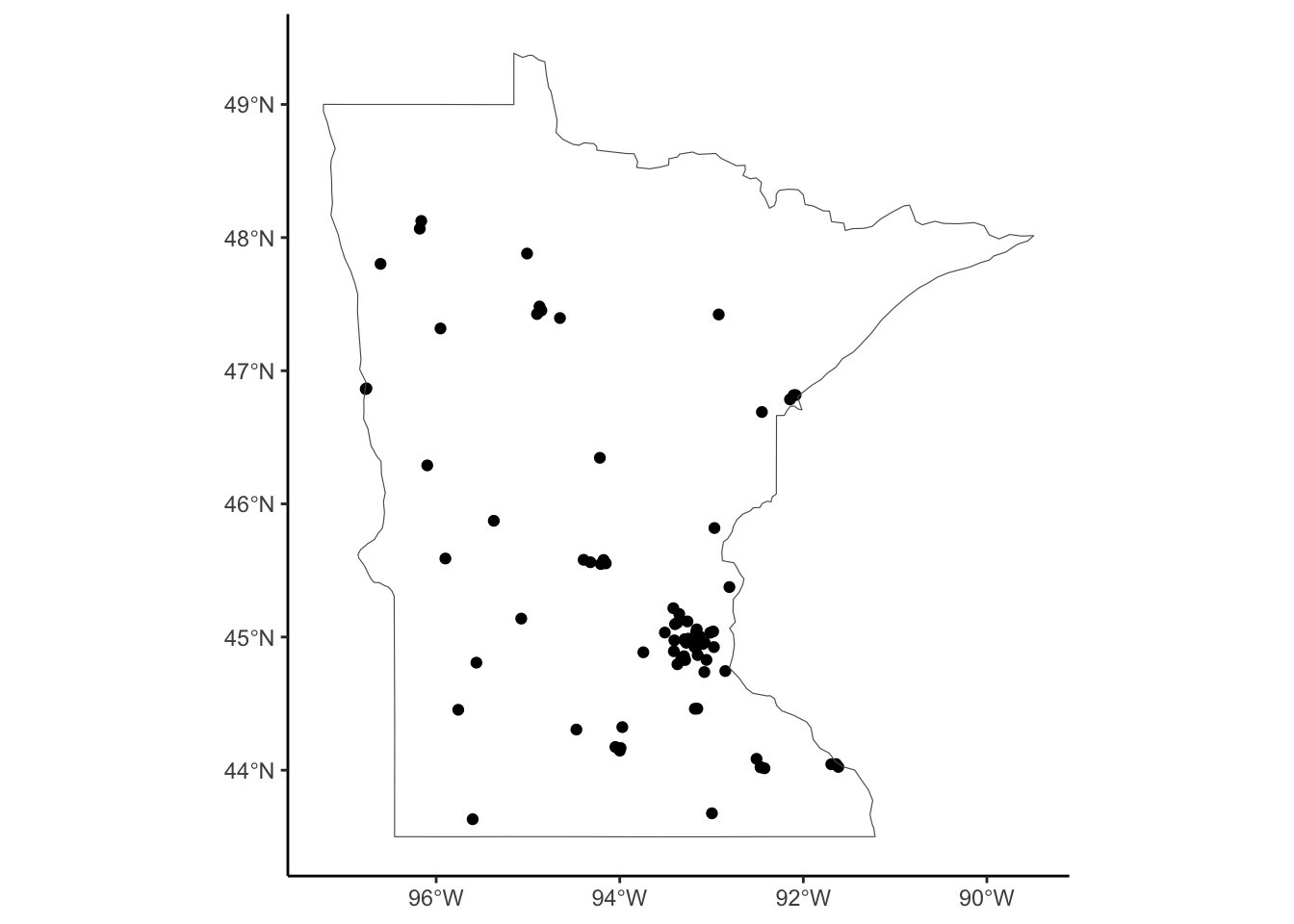
We can plot these points by passing the data set to ggplot() and use geom_sf() to plot the geometry list in the appropriate form (point, line, polygon, etc.). Go ahead and plot the locations of the colleges and universities in MN.
colleges %>%filter(STABBR =='MN') %>% ??
Spatial Polygons
If we’d like the state boundaries, we’ll need to get the those values as a polygon. Thankfully, the USAboundaries package has all of that information for us.
Notice the geometry type and also note the CRS (Coordinate Reference System).
In order to plot the points of the colleges on the same plot as the polygons of state boundaries, we need to make sure we are using the same CRS. You might have noticed that the colleges data set didn’t have a CRS listed, so let’s set the CRS of colleges to be the same as the states.
st_crs(colleges) <-st_crs(states) # provide CRS, if it doesn't have an existing CRS
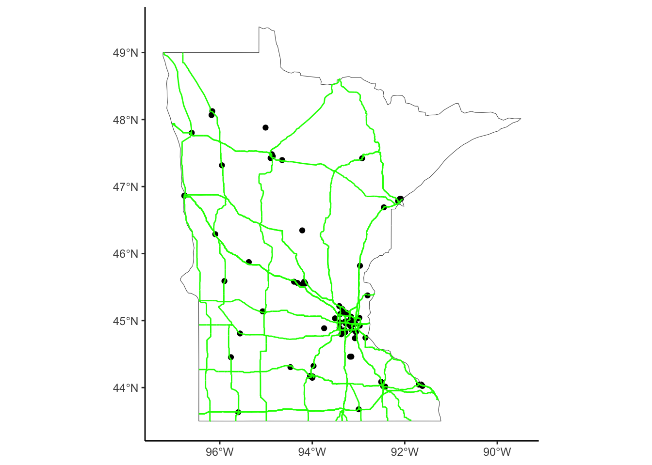
Add to your existing plot of college locations by adding + geom_sf(data = states %>% filter(state_name == 'Minnesota'), alpha = 0). Notice how it knows what type of plot to make based on the geometry type.
roads <-read_sf('tl_2019_27_prisecroads')roads <-st_transform(roads, crs =st_crs(states)) # change CRS if it has an existing CRSroads
Now that we have this spatial data set loaded, let’s add to our previous plot by adding + geom_sf(data = roads %>% filter(RTTYP %in% c('U','I')), color = 'green'). In this codoe, we are first filtering the roads data set to only include U.S. State roads and Interstate highways and coloring them green.
We’ve worked with spatial points, lines, and polygons. So far, we’ve focused only on locations. These plots do not encode any outcome data.
Mapping Data
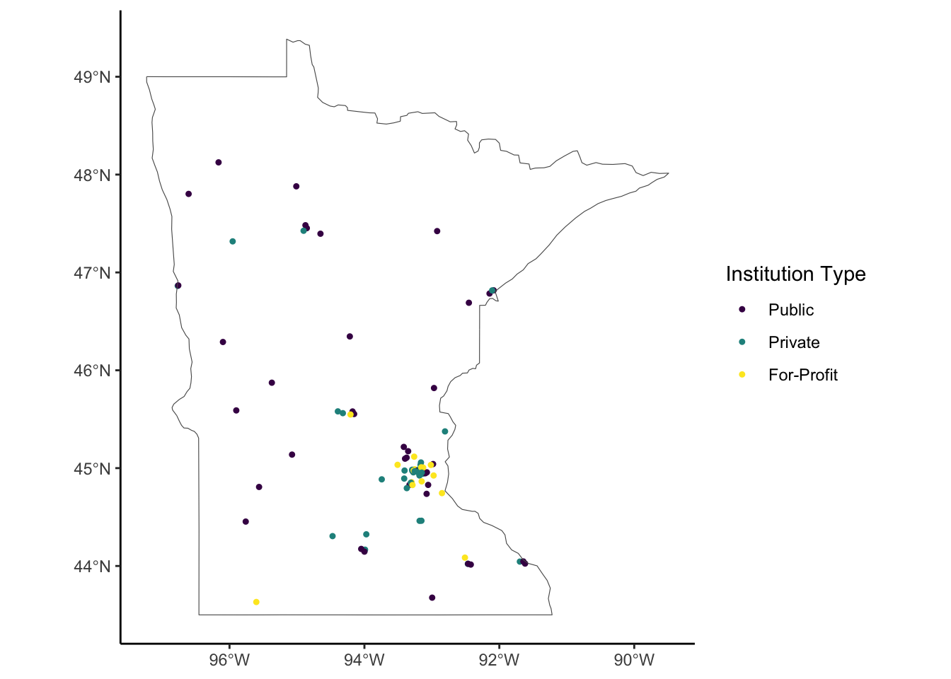
Think about how might you be able to incorporate the CONTROL of the college (1: Public, 2: Non-Profit Private, 3: For-Profit Private). Try creating a graph with that outcome data visualized on the map.
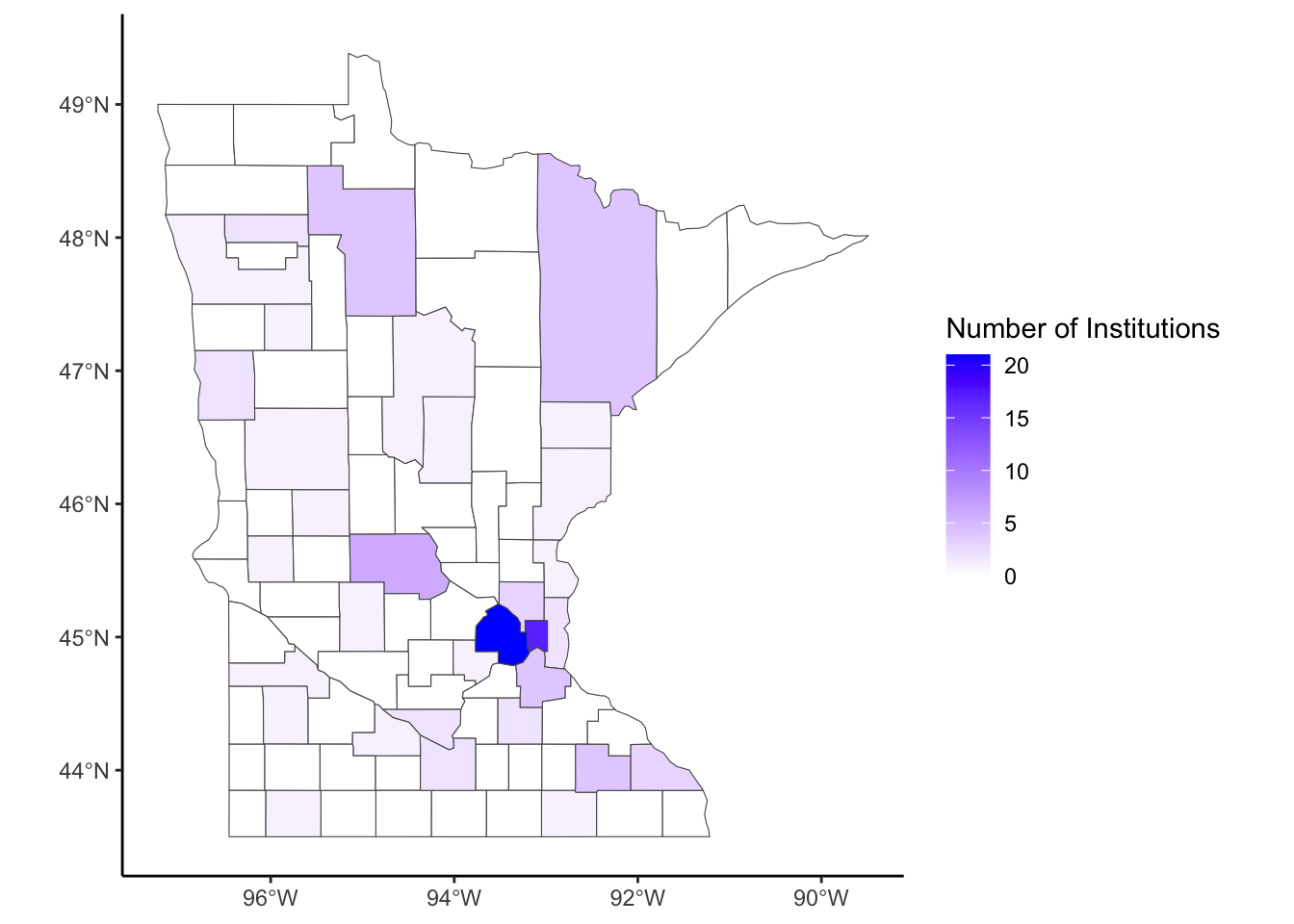
Let’s consider counties in MN. What if we wanted to aggregate the college information (such as # of colleges) to a county level?
countiesMN <-us_counties(states ='MN') # get counties in MNhead(countiesMN)
We want to check to see how many colleges are in each county. You can use st_intersects(X,Y) to check to see if the geometry of X intersects with the geometry of Y. In other words, we want to see for each county how many MN college point locations are in the county polygon.
sf::sf_use_s2(FALSE) # avoids an error with spherical geometry.# Counts the number of points (colleges) that intersect with each polygon (counties)countiesMN <- countiesMN %>%mutate(NumColleges =st_intersects(countiesMN, colleges %>%filter(STABBR =='MN')) %>%lengths())##Create a plot of counties and fill according to the number of collegescountiesMN %>% ???
Solutions
Small Group Work
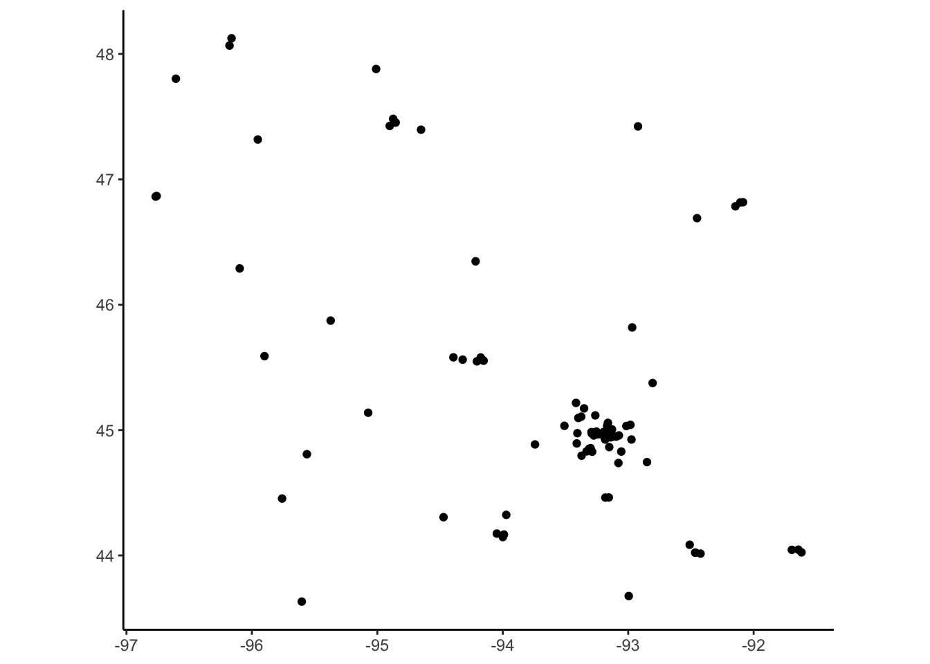
Spatial Points
Solution
These are POINTS!
Simple feature collection with 6 features and 70 fields
Geometry type: POINT
Dimension:     XY
Bounding box:  xmin: -87.52959 ymin: 32.36261 xmax: -86.17401 ymax: 34.78337
CRS:           NA
# A tibble: 6 × 71
  UNITID INSTNM      IALIAS ADDR  CITY  STABBR ZIP    FIPS OBEREG CHFNM CHFTITLE
   <dbl> <chr>       <chr>  <chr> <chr> <chr>  <chr> <dbl>  <dbl> <chr> <chr>
1 100654 Alabama A … AAMU   4900… Norm… AL     35762     1      5 Dr. … Preside…
2 100663 University… UAB    Admi… Birm… AL     3529…     1      5 Ray … Preside…
3 100690 Amridge Un… South… 1200… Mont… AL     3611…     1      5 Mich… Preside…
4 100706 University… UAH  … 301 … Hunt… AL     35899     1      5 Chuc… Preside…
5 100724 Alabama St… <NA>   915 … Mont… AL     3610…     1      5 Quin… Preside…
6 100733 University… <NA>   500 … Tusc… AL     35401     1      5 Sid … Interim…
# ℹ 60 more variables: GENTELE <dbl>, EIN <chr>, UEIS <chr>, OPEID <chr>,
#   OPEFLAG <dbl>, WEBADDR <chr>, ADMINURL <chr>, FAIDURL <chr>, APPLURL <chr>,
#   NPRICURL <chr>, VETURL <chr>, ATHURL <chr>, DISAURL <chr>, SECTOR <dbl>,
#   ICLEVEL <dbl>, CONTROL <dbl>, HLOFFER <dbl>, UGOFFER <dbl>, GROFFER <dbl>,
#   HDEGOFR1 <dbl>, DEGGRANT <dbl>, HBCU <dbl>, HOSPITAL <dbl>, MEDICAL <dbl>,
#   TRIBAL <dbl>, LOCALE <dbl>, OPENPUBL <dbl>, ACT <chr>, NEWID <dbl>,
#   DEATHYR <dbl>, CLOSEDAT <chr>, CYACTIVE <dbl>, POSTSEC <dbl>, …
Here are all of the colleges in MN plotted as points.
Spatial Polygons
Solution
Spatial Lines
Solution
Simple feature collection with 6 features and 4 fields
Geometry type: LINESTRING
Dimension:     XY
Bounding box:  xmin: -95.91068 ymin: 44.77785 xmax: -93.39901 ymax: 45.58255
Geodetic CRS:  WGS 84
# A tibble: 6 × 5
  LINEARID      FULLNAME         RTTYP MTFCC                            geometry
  <chr>         <chr>            <chr> <chr>                    <LINESTRING [°]>
1 110448792990  US Hwy 59 Byp    U     S1200 (-95.90696 45.57834, -95.9073 45.5…
2 110448792980  State Hwy 59 Byp S     S1200 (-95.90196 45.57331, -95.90296 45.…
3 1104271370555 Shakopee Byp     M     S1200 (-93.55982 44.7781, -93.55951 44.7…
4 1108296486854 Shakopee Byp     M     S1100 (-93.39901 44.79892, -93.39906 44.…
5 1105577101570 Paynesville Byp  M     S1200 (-94.78041 45.35509, -94.78182 45.…
6 1104295165103 Shakopee Byp     M     S1200 (-93.55981 44.77785, -93.5595 44.7…
Mapping Data
.
Solution
.
Solution
Simple feature collection with 6 features and 15 fields
Geometry type: MULTIPOLYGON
Dimension:     XY
Bounding box:  xmin: -96.78579 ymin: 43.50018 xmax: -93.01956 ymax: 46.63078
Geodetic CRS:  WGS 84
    statefp countyfp countyns       affgeoid geoid     name        namelsad
16       27      059 00659475 0500000US27059 27059   Isanti   Isanti County
26       27      165 00659527 0500000US27165 27165 Watonwan Watonwan County
60       27      023 00659457 0500000US27023 27023 Chippewa Chippewa County
92       27      149 00659519 0500000US27149 27149  Stevens  Stevens County
160      27      091 00659490 0500000US27091 27091   Martin   Martin County
226      27      167 00659528 0500000US27167 27167   Wilkin   Wilkin County
    stusps state_name lsad      aland   awater state_name_2 state_abbr
16      MN  Minnesota   06 1128608895 41203099    Minnesota         MN
26      MN  Minnesota   06 1126508687 12387832    Minnesota         MN
60      MN  Minnesota   06 1505378148 17239137    Minnesota         MN
92      MN  Minnesota   06 1459664592 30322218    Minnesota         MN
160     MN  Minnesota   06 1844928076 44669373    Minnesota         MN
226     MN  Minnesota   06 1945179856   480470    Minnesota         MN
    jurisdiction_type                       geometry
16              state MULTIPOLYGON (((-93.51368 4...
26              state MULTIPOLYGON (((-94.8598 44...
60              state MULTIPOLYGON (((-96.0367 45...
92              state MULTIPOLYGON (((-96.25402 4...
160             state MULTIPOLYGON (((-94.85444 4...
226             state MULTIPOLYGON (((-96.78579 4...
Wrap-Up
Finishing the Activity
If you didn’t finish the activity, no problem! Be sure to complete the activity outside of class, review the solutions in the online manual, and ask any questions on Slack or in office hours.
Re-organize and review your notes to help deepen your understanding, solidify your learning, and make homework go more smoothly!
After Class
Before the next class, please do the following:
Take a look at the Schedule page to see how to prepare for the next class.