8.4 Continuous Random Variables
For continuous random variables \(X\) (uncountable, infinite number of values),
the probability of any one value is 0, \(P(X = x) = 0\).
So we define the probability model using a culmulative distribution function (cdf), the probability of having a value less than \(x\), \[F(x) = P(X\leq x)\] (it is always notated with a capital letter \(F\) or \(G\) or \(H\)).
and a probability density function (pdf), \(f(x)\geq 0\) such that the probability is defined by the area under this curve (defined by the pdf). Using calculus, the area under the curve is \[P(a\leq X \leq b) = \int^b_a f(x)dx\] (it is always notated with a small letter \(f\) or \(g\) or \(h\)) and the total area under the probability density function is 1, \[P(S) = P(-\infty\leq X\leq \infty) = \int^\infty_{-\infty}f(x)dx = 1\]
Thus, we can write the cumulative distribution function as, \(F(x) = P(X \leq x) = \int^x_{-\infty} f(y)dy\).
8.4.1 Expected Value
Let \(X\) be a continuous RV with pdf \(f(x)\). The expected value of \(X\) is defined as \[E(X)= \int^\infty_{-\infty} xf(x)dx \] and \[E(g(X))= \int^\infty_{-\infty} g(x)f(x)dx\]
Properties of Expected Value
These properties still hold:
\[ E(aX) = aE(X)\] \[E(X+b) = E(X) + b\]
8.4.2 A Few Named Probability Models
Normal Model
For \(X\) such that \(E(X) = \mu\) and \(SD(X) = \sigma\), a Normal random variable has a pdf of \[f(x) = \frac{1}{\sigma\sqrt{2\pi}}e^{-\frac{(x-\mu)^2}{2\sigma^2}}\]
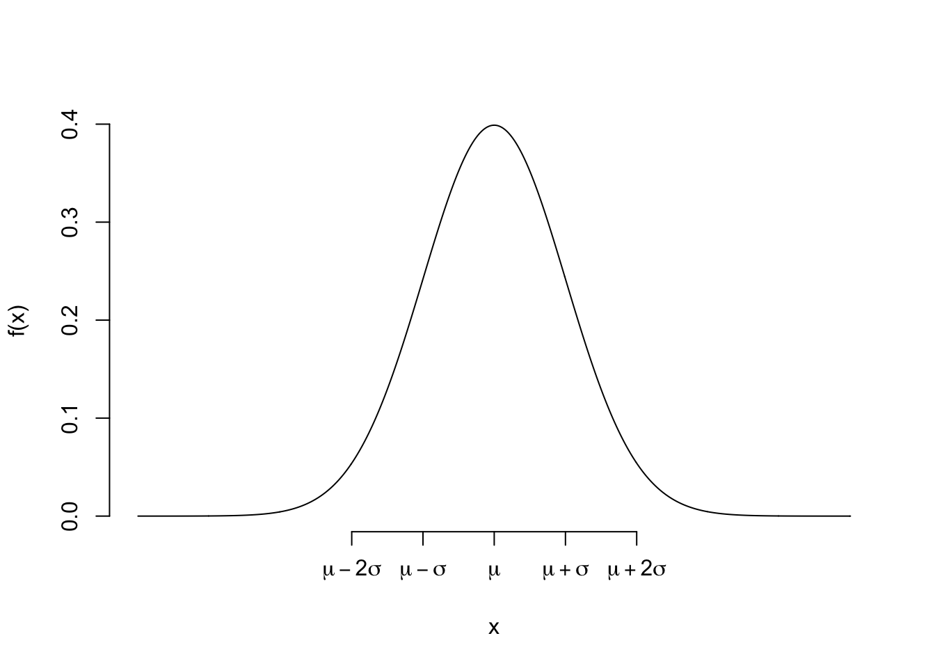
Let the expected value be 0 and standard deviation be 1, \(\mu = 0\) and \(\sigma = 1\)
We know that \(P(-1\leq X \leq 1) = F(1) - F(-1) = 0.68\)
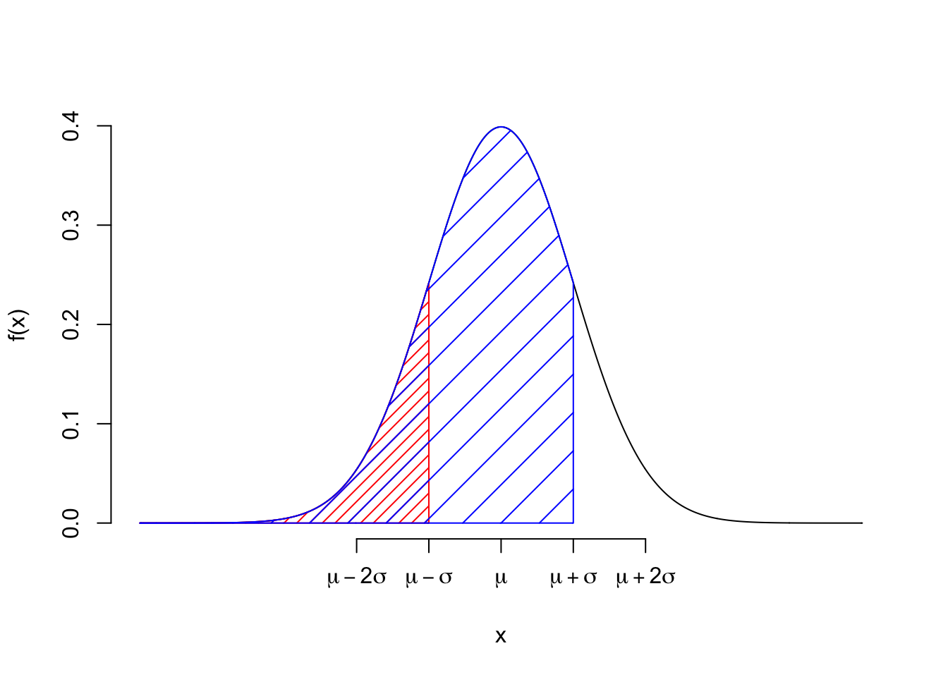
## [1] 0.6826895- \(P(-2\leq X \leq 2) = F(2) - F(-2) = 0.95\)
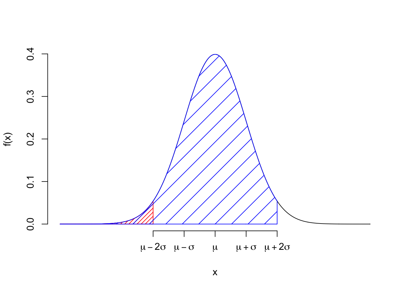
## [1] 0.9544997- \(P(-3\leq X \leq 3) = F(3) - F(-3) = 0.997\)
## [1] 0.9973002Let \(X\) be a Binomial Random Variable and \(Y\) be a Normal Random Variable.
As \(n\rightarrow \infty\) (\(p\) is fixed), the \(P(X = x) \approx P(x-0.5 \leq Y \leq x+0.5)\).
Note: adding and subtracting 0.5 is the continuity correction
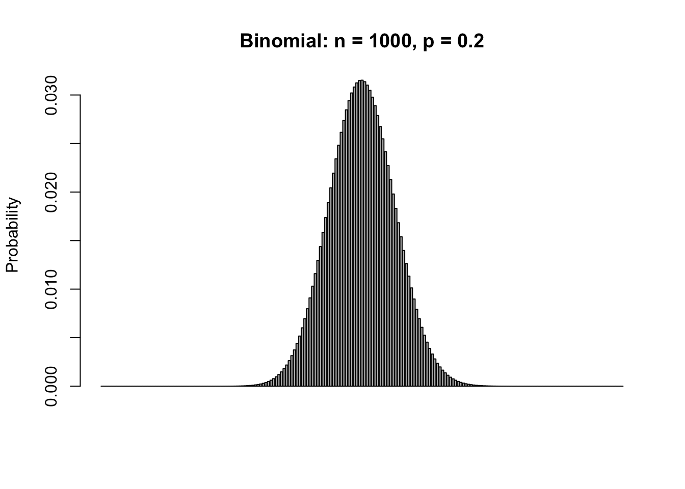
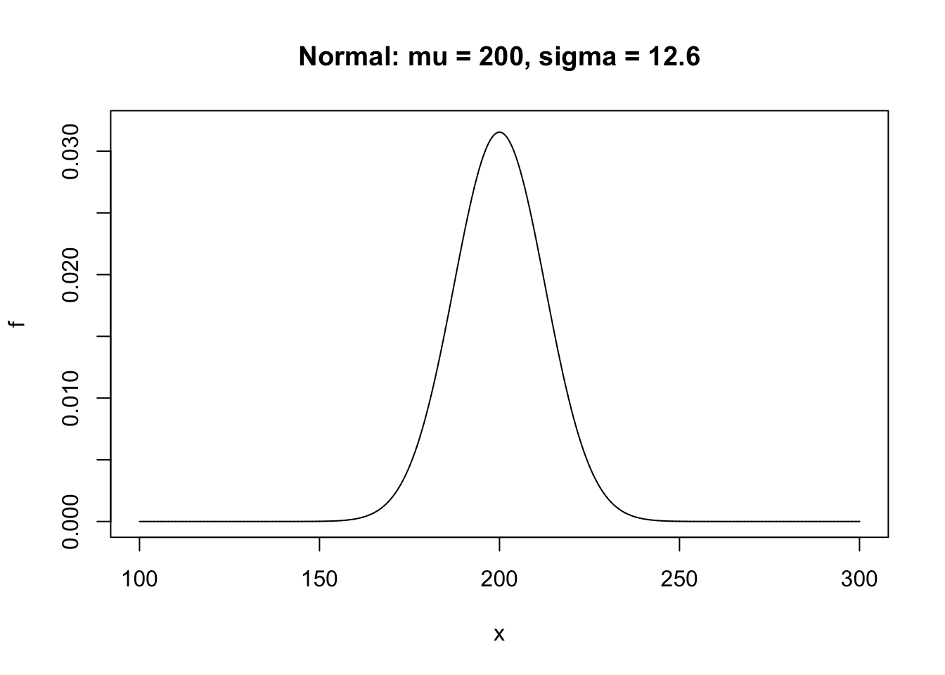
If \(n=1000\) and \(p=0.2\), let’s compare \(P(X=200)\) and \(P(199.5\leq Y\leq 200.5)\).
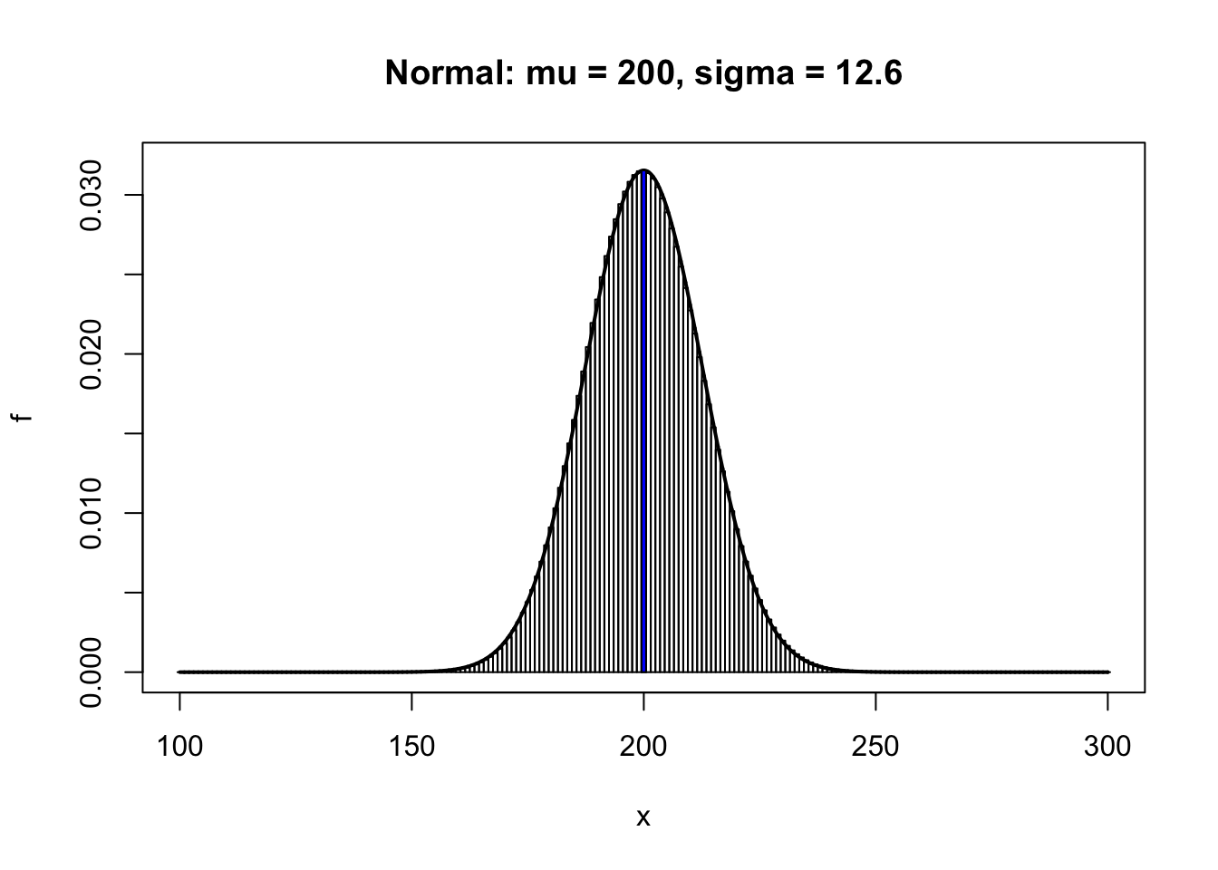
## [1] 0.03152536## [1] 0.03153095If \(n=1000\) and \(p=0.2\), let’s compare \(P(200\leq X\leq 210)\) and \(P(199.5\leq Y\leq 210.5)\).
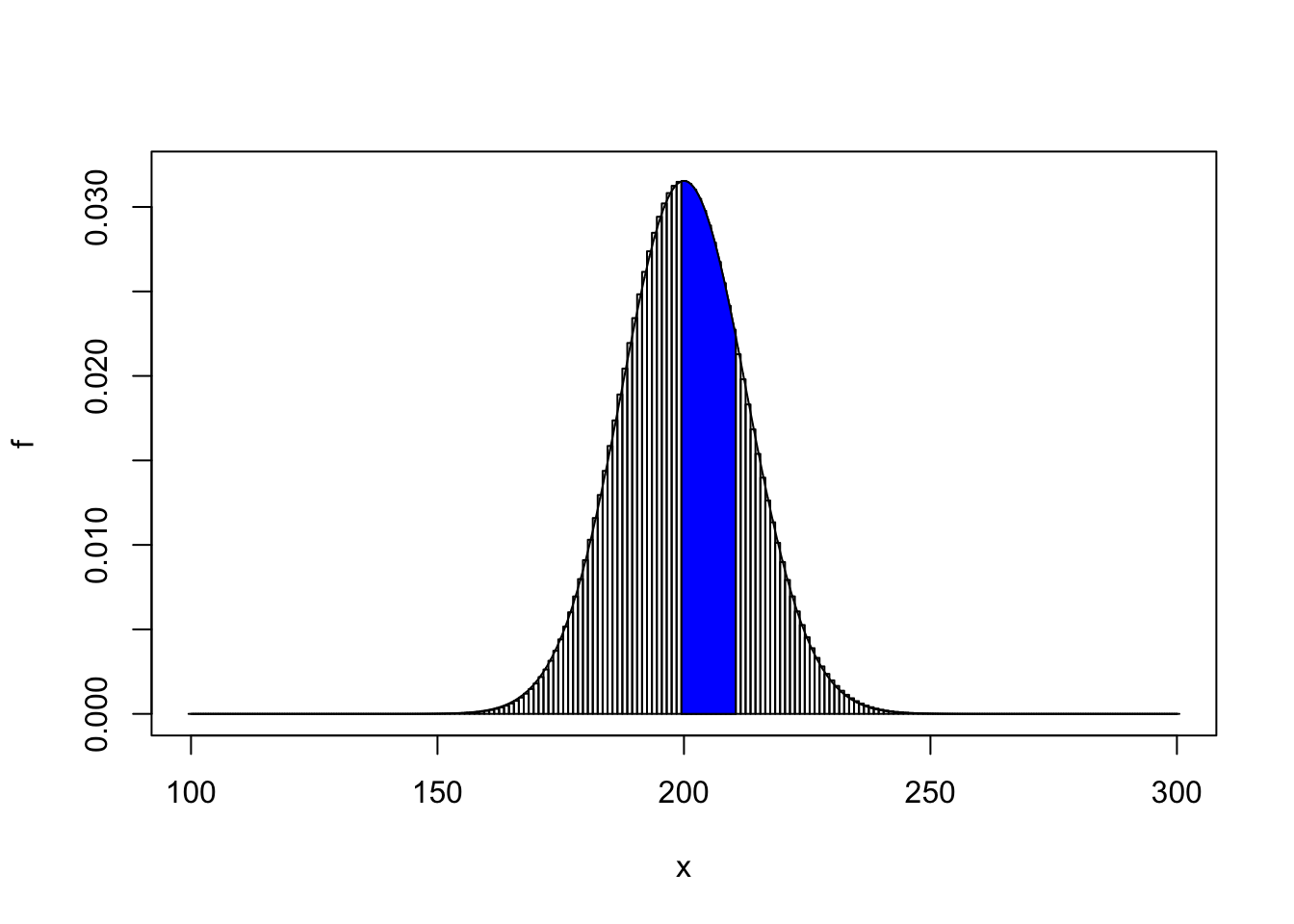
## [1] 0.3100719## [1] 0.3125238How big does \(n\) have to be for the Normal approximation to be appropriate?
- Rule of Thumb: \(np \geq 10\) and \(n(1-p)\geq 10\) because that makes sure that \(E(X)-0>3SD(X)\) (mean is at least 3 SD’s from 0).
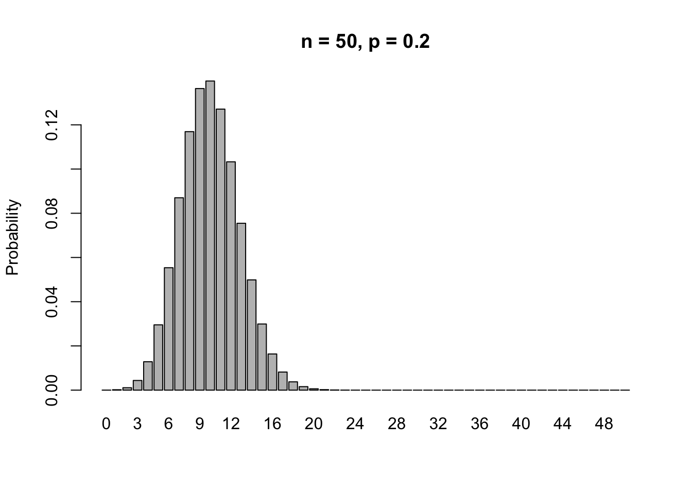
For \(p=0.2\), that means that \(n\geq 50\).
n = 50
p = 0.2
barplot(dbinom(0:n,size = n, p = p),names.arg=0:n,ylab='Probability',main='n = 50, p = 0.2')