3.6 Model Interpretation
Let’s look at the summary output of the lm() function in R again. We’ll highlight some of the most important pieces of this output and discuss how you interpret them.
## # A tibble: 2 x 5
##   term        estimate std.error statistic  p.value
##   <chr>          <dbl>     <dbl>     <dbl>    <dbl>
## 1 (Intercept)    -3.19     5.50     -0.580 5.62e- 1
## 2 Neck            2.74     0.145    18.9   4.59e-50
3.6.1 Intercept (\(\hat{\beta}_0\))
- Where to find: In the table called “Coefficients”, look for the number under “Estimate” for “(Intercept)”. It is -3.1885 for this model.
- Definition: The intercept gives the average value of \(y\) when \(x=0\) (think about context)
- Interpretation: If Neck size = 0, then the person doesn’t exist. In this context, the intercept doesn’t make much sense to interpret.
- Discussion: If the intercept doesn’t make sense in the context, we might refit the model with the \(x\) variable once it is centered. That is, the mean of \(x\) for all individuals in the sample is computed, and this mean is subtracted from each person’s \(x\) value. In this case, the intercept is interpreted as the average value of \(y\) when \(x\) is at its (sample) mean value. See the example below – we get an intercept of 100.66, which is the average Chest size for customers with average Neck size. We could also choose to center Neck size at a value other than the mean. For example, we could center it at 30 cm by subtracting 30 from the Neck size of all cases.
body <- body %>%
  mutate(CNeck = Neck - mean(Neck))

tshirt_mod2 <- body %>%
  with(lm(Chest ~ CNeck))

tshirt_mod2 %>%
  tidy()
## # A tibble: 2 x 5
## term estimate std.error statistic p.value
## <chr> <dbl> <dbl> <dbl> <dbl>
## 1 (Intercept) 101. 0.330 305. 3.14e-321
## 2 CNeck 2.74 0.145 18.9 4.59e- 503.6.2 Slope (\(\hat{\beta}_1\))
- Where to find: In the table called “Coefficients”, look for the number under “Estimate” for the name of the variable, “Neck” or “CNeck”. It is 2.7369 for this model. (Note: the slopes for both
tshirt_modandtshirt_mod2are the same. Why?) - Definition: The slope gives the change in average \(y\) per 1 unit increase in \(x\) (not for individuals and not a causal statement)
- One Interpretation: If we compare two groups of individuals with a 1 cm difference in the neck size (e.g., 38 cm and 39 cm OR 40 cm and 41 cm), then we’d expect the average chest sizes to be different by about 2.7 cm.
- Another Interpretation: We’d expect the average chest size to increase by about 2.7 cm for each centimeter increase in neck size.
- A Third Interpretation: We estimate that a one centimeter increase in neck size is associated with an increase, on average, of 2.7 cm in chest size.
- Discussion: Note that the interpretations are not written about an individual because the least squares line (our fit model) is a description of the general trend in the population. The slope describes the change in the average, not the change for one person.
3.6.3 Least Squares Regression Line (\(\hat{y} = \hat{\beta}_0 + \hat{\beta}_1x\))
- Where to find: In the table called “Coefficients”, all of the values that you need to write down the formula of the line are in the “Estimate” column.
- Definition: The line gives the estimated average of \(y\) for each value of \(x\) (within the observed range of x)
- Interpretation: The fit regression line of (Predicted Chest = -3.18 + 2.73*Neck) gives the estimated average Chest size for a given Neck size, based on our sample of data.
- Discussion: The “within the observed range of \(x\)” phrase is very important. We can’t predict values of \(y\) for values of \(x\) that are very different from what we have in our data. Trying to do so is a big no-no called extrapolation. We’ll discuss this more in a bit.
3.6.4 Correlation vs. Causation
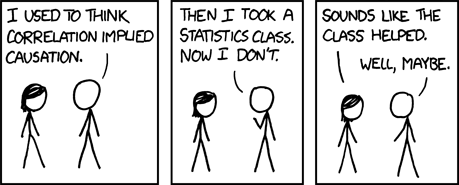 Source: xkcd
What is causation? What is a causal effect? Are there criteria for defining a cause?
These are deep questions that have been debated by scientists of all domains for a long time. We are at a point now where there is some consensus on the definition of a causal effect. The causal effect of a variable \(X\) on another variable \(Y\) is the amount that we expect \(Y\) to change if we intervene on or manipulate \(X\) by changing it by one unit.
When can we interpret an estimated slope, \(\hat{\beta}_1\), from a simple linear regression as a causal effect of \(X\) on \(Y\)? Well, in the simple linear regression case, almost never. To interpret the slope as a causal effect, there would have to be no confounding variables (no variables that cause both \(X\) and \(Y\)). If we performed an experiment, it might be possible to have no confounding variables, but in most situations, this is not feasible.
Then what are we to do?
- Think about the possible causal pathways and try and create a DAG (coming up - see Section 3.11).
- Try to adjust or control for possible confounders using multiple linear regression by including them in the model (coming up - see Section 3.9).
- After fitting a model, we should step back and consider other criteria such as Hill’s Criteria before concluding there is a cause and effect relationship. Think about whether there is a large effect, whether it can be reproduced in another sample, whether the the effect happens before the cause in time, etc.