8.3 Discrete Random Variables
If there are a finite (more generally, countable) number of possible values, we say that \(X\) is a discrete random variable.
We often can write the probability as a function of values, \(x\), and we call this function the probability mass function (pmf), \[p(x) = P(X = x)\]
and we know that \[\sum_{all~x}p(x) = 1\]
8.3.1 Expected Value
The expected value (or long-run average) of a discrete random variable is defined as the weighted average of the possible values, weighted by the probability,
\[E(X) = \sum_{all~x} xp(x)\]
So the expected value is like a mean, but over the long-run.
8.3.2 Variance
The variance (or long-run spread) of a discrete random variable is defined as the “average” squared distance of \(X\) from its expected value,
\[Var(X) = E[(X-\mu)^2]\] where \(\mu = E(X)\).
- But it’s in squared units, so typically we talk about its square root, called the standard deviation of a random variable, \[SD(X) = \sqrt{Var(X)}\]
So the standard deviation of a random variable is like the standard deviation of a set of observed values. They are measures of spread and variability. In one circumstance, we have the data to calculate it and in the other, we are considering a random process and wondering how much a value might vary.
8.3.3 Joint Distributions
The joint probability mass function for two random variables is \[p(x,y) = P(X=x \text{ and }Y = y)\]
We can often calculate this joint probability using our probability rules from above (using multiplication…)
The expected value for a function of two random variables is \[E(g(X,Y)) = \sum_{all\; y}\sum_{all\; x} g(x,y)p(x,y)\]
We could show that the expected value of a sum is the sum of the expected values:
\[E(X+Y) = E(X) + E(Y)\]
- Using this fact, we could show that the variance can be written in this alternative form:
\[Var(X) = E[(X-\mu)^2] = E(X^2) - [E(X)]^2\]
8.3.4 Covariance
When consider two random variables, we may wonder whether they co-vary? In that do they vary together or vary independently? If
The covariance of two random variables is defined as \[Cov(X,Y) = E[(X - \mu_X)(Y - \mu_Y)] = E(XY) - E(X)E(Y)\]
Note: The covariance of X with itself is just the variance, \(Cov(X,X) = Var(X)\)
We could use this to show that \(Var(X+Y) = Var(X)+ Var(Y) + 2Cov(X,Y)\).
Two discrete random variables are independent if and only if \[P(X = x\text{ and } Y = y) = P(X=x)P(Y=y)\] for every \(x\) and \(y\).
- If two random variables, \(X\) and \(Y\) are independent, then \(Cov(X,Y)= 0\).
8.3.5 Correlation
- The correlation of two random variables is \[Cor(X,Y) =\frac{Cov(X,Y)}{SD(X)SD(Y)}\]
8.3.6 A Few Named Probability Models
8.3.6.1 Bernoulli Trials
Three conditions
- Two possible outcomes on each trial (success or failure)
- Independent Trials (result of one trial does not impact probabilities on next trial)
- P(success) = \(p\) is constant
\[P(X = x) = p^x (1-p)^{x-1} \text{ for } x\in\{0,1\}\] \[E(X) = p\] \[Var(X) = p(1-p) \]
Binomial RV: \(X\) is the total number of successes in \(n\) trials
For general \(n\) and \(x\), the Binomial probability for a particular value of \(x\) is given by
\[P(X = x) =\frac{n!}{(n-x)! x!} p^x (1-p)^{n-x}\text{ for } x\in\{0,1,2,...,n\}\] where \(x! = x*(x-1)*(x-2)*\cdots*2*1\) and \(0! = 1\), so
\[\frac{n!}{(n-x)! x!} = \frac{n*(n-1)*\cdots*(n-x+1)*(n-x)!}{(n-x)! x!}\] \[= \frac{n*(n-1)*\cdots*(n-x+1)}{x*(x-1)*\cdots*2*1}\]
If we break this apart, we can see where the pieces came from. Let’s consider a simplified example. Let \(X\) be the number of Heads in 3 coin flips (but the coin is biased such that \(p=0.2\)).
The probability of \(2\) successes and \(1\) failure in one particular order (e.g. HHT) is calculated as \(p^x (1-p)^{n-x} = 0.2^2(0.8)\) due to Rule 5. However, we could have gotten a different ordering of Heads and Tails (e.g. HTH, THH). To count the number of ways we could get 2 heads and 1 tail in 3 coin flips, we use tools from combinatorics (an area of mathematics). In fact, the first part of the equation does the counting for us,
\[\frac{n!}{(n-x)! x!} = \frac{n*(n-1)*\cdots*(n-x+1)*(n-x)!}{(n-x)! x!}\]
So for our example, there are \(\frac{3!}{2!1!} = \frac{3*2!}{2!1} = 3\) orderings of 2 heads and 1 tail.
The expected number of successes in the long run is
\[E(X) = np\] and the variability in the number of successes is given by
\[Var(X) = np(1-p) \]
Let’s plot the pmf of the Binomial in a bar plot,
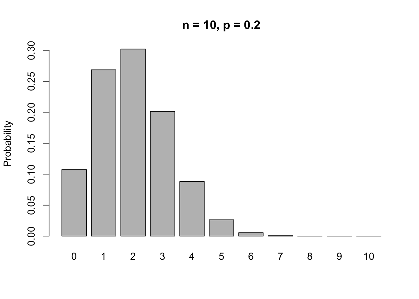
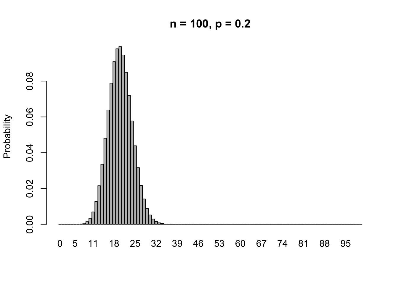
If we increase \(n\), but leave \(p\), then
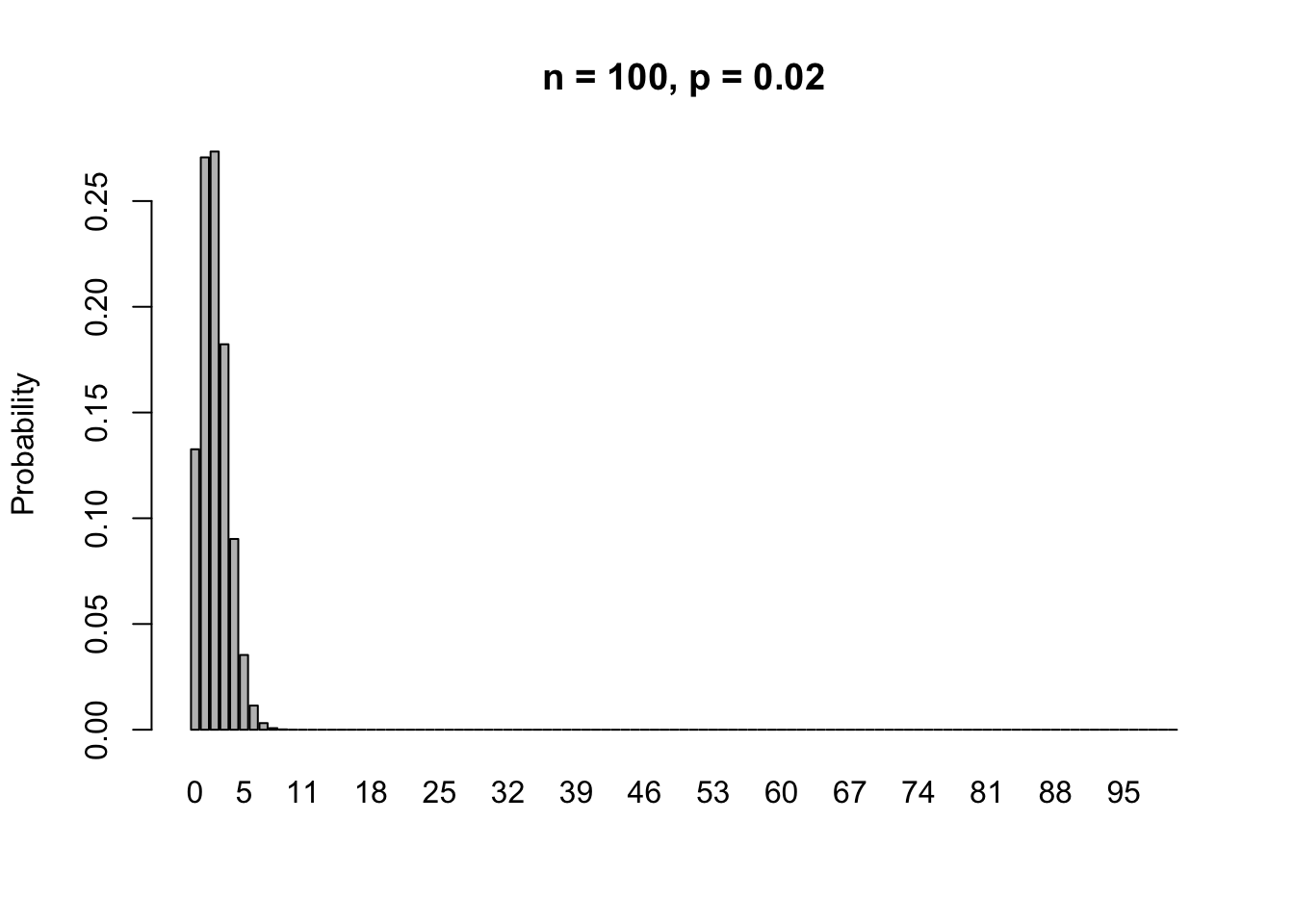
If we increase \(n\), but decrease \(p\) proportionally (such that \(np\) stays the same), then
We will talk about two ways to approximate the Binomial distribution.
- If \(n\) increases while \(p\) stays fixed, then we use a Normal approximation.
- If \(n\) increases and \(p\) decreases, then we use a Poisson approximation (beyond the scope of this course).