4.4 Logistic Model Prediction
On January 28, 1986, the temperature was 26 degrees F. Let’s predict the chance of “success,” which is a failure of o-rings in our data context, at that temperature.
#type = 'response' gives predicted chance, rather than predicted odds
predict(model.glm, newdata = data.frame(Temperature = 26), type = 'response')
## 1
## 0.9998774They didn’t have any experimental data testing o-rings at this low of temperatures, but even based on the data collected, we predict the chance of failure to be nearly 1 (near certainty).
4.4.1 Hard Predictions/Classifications
These predicted chances of “success” are useful to give us a sense of uncertainty in our prediction. If the chance of o-ring failure were 0.8, we would be fairly certain that a failure were likely but not absolutely. If the chance of o-ring failure were 0.01, we would be pretty certain that a failure was not likely to occur.
But if we had to decide whether or not we should let the shuttle launch go, how high should the predicted chance be to delay the launch (even if it would cost a lot of money to delay)?
It depends. Let’s look at a boxplot of predicted probabilities of “success” compared to the true outcomes.
model.glm %>%
  augment(type.predict = 'response') %>%
  ggplot(aes(x = factor(Fail), y = .fitted)) +
  geom_boxplot() +
  labs(y = 'Predicted Probability of Outcome', x = 'True Outcome') +
  theme_classic()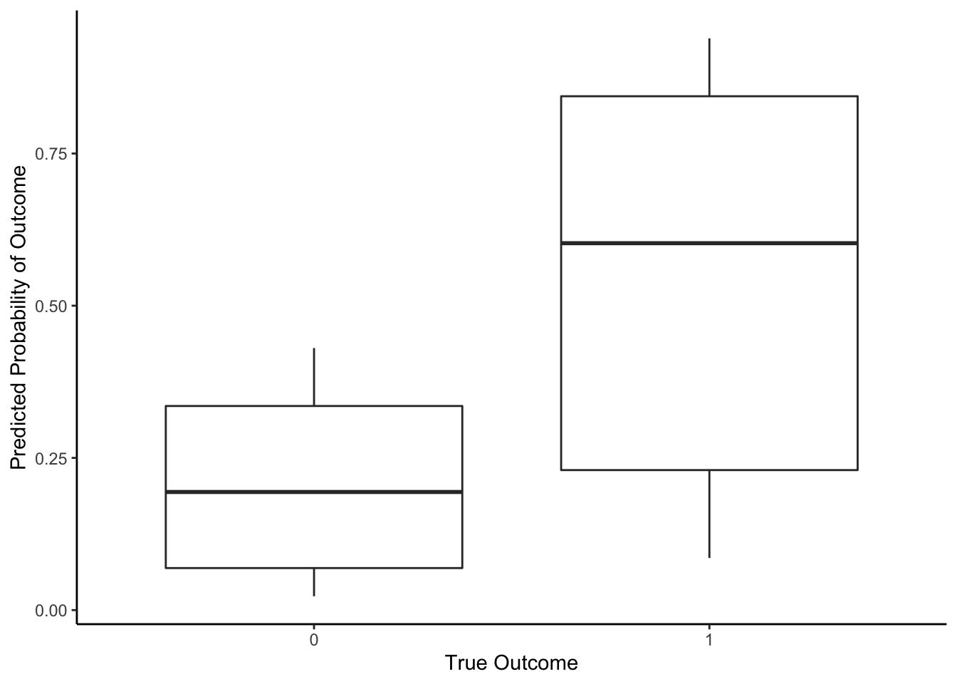
If we used a threshold of 0.8, then we’d say that for any experiment with a predicted chance of o-ring failure 0.8 or greater, we’ll predict that there will be o-ring failure. As with any predictions, we may make an error. With this threshold, what is our accuracy (# of correctly predicted/# of data points)?
model.glm %>%
  augment(type.predict = 'response') %>%
  ggplot(aes(x = factor(Fail), y = .fitted)) +
  geom_boxplot() +
  labs(y = 'Predicted Probability of Outcome', x = 'True Outcome') +
  geom_hline(yintercept = 0.8, color = 'red') + #threshold
  theme_classic()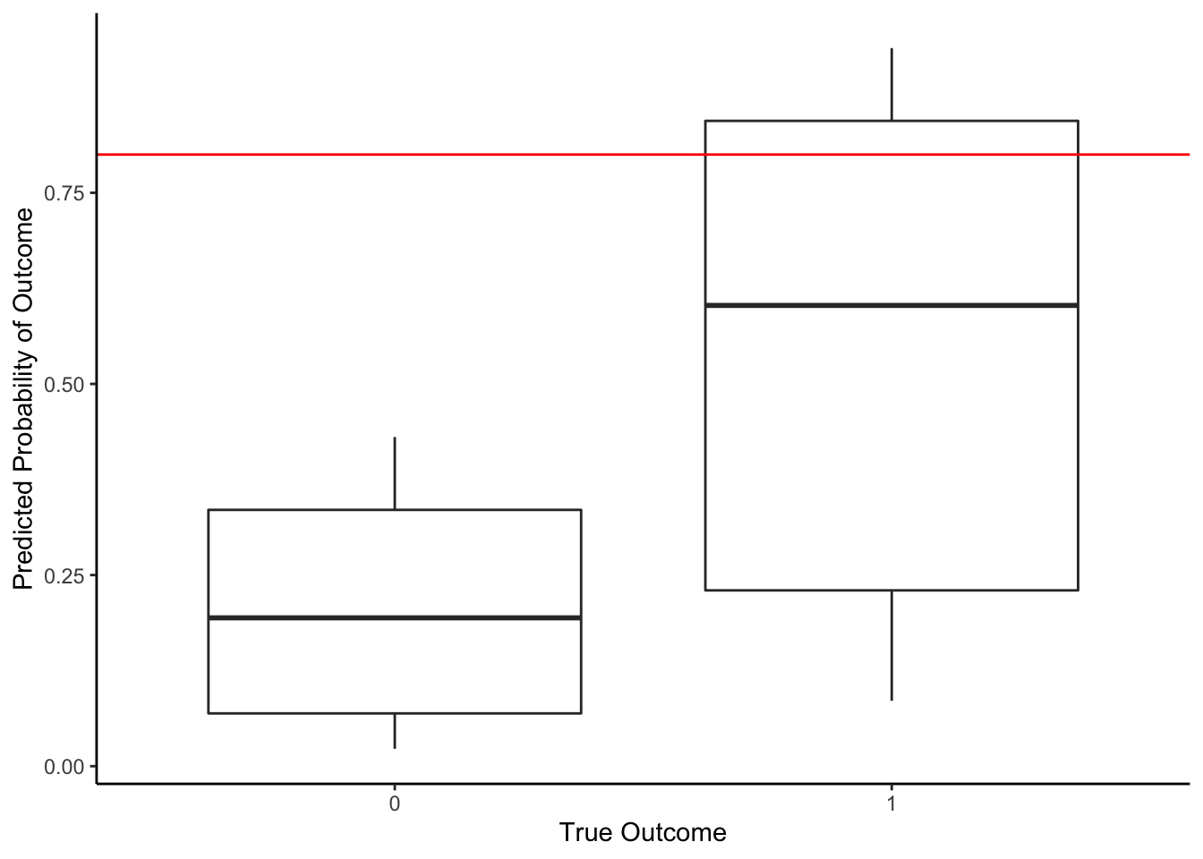
In the table below, we see that there were 3 data points in which we correctly predicted o-ring failure (using a threshold of 0.8). There were 4 data points in which we erroneously predicted that it wouldn’t fail when it actually did, and we correctly predicted no failure for 16 data points. So in total, our accuracy is (16+3)/(16+4+3) = 0.82 or 82%.
threshold <- 0.80

model.glm %>%
  augment(type.predict ='response') %>%
  mutate(predictFail = .fitted >= threshold) %>%
  count(Fail, predictFail) %>%
  mutate(correct = (Fail == predictFail)) %>%
  group_by(Fail) %>%
  mutate(prop = n/sum(n)) #Specificity, False pos, False neg, Sensitivity
## # A tibble: 3 x 5
## # Groups: Fail [2]
## Fail predictFail n correct prop
## <dbl> <lgl> <int> <lgl> <dbl>
## 1 0 FALSE 16 TRUE 1
## 2 1 FALSE 4 FALSE 0.571
## 3 1 TRUE 3 TRUE 0.429The only errors we made were false negatives (predict no “success” because \(\hat{p}\) is less than threshold when outcome was true “success”, \(Y=1\)); we predicted that the o-ring wouldn’t fail but the o-rings did fail in the experiment (\(Y=1\)). In this data context, false negatives have real consequences on human lives because a shuttle would launch and potentially explode because we had predicted there would be no o-ring failure.
The false negative rate is the number of false negatives divided by the false negatives + true positives (denominator should be total number of experiments with actual o-ring failures). With a threshold of 0.80, our false negative rate is 4/(3+4) = 0.57 = 57%. We failed to predict 57% of the o-ring failures. This is fairly high when there are lives on the line.
The sensitivity of a prediction model is the true positives divided by the false negatives + true positives (denominator should be total number of experiments with actual o-ring failures). It is 1-false negative rate, so the model for o-ring failures has a 1-0.57 = 0.43 or 43% sensitivity.
A false positive (predict “success” because \(\hat{p}\) is greater than threshold when outcome was not a “success”, \(Y=0\)). A false positive would happen when we predicted o-ring failure when it doesn’t actually happen. This would delay launch (cost $) but have minimal impact on human lives.
The false positive rate is the number of false positives divided by the false positives + true negatives (denominator should be total number of experiments with no o-ring failures). With a threshold of 0.80, our false positive rate is 0/16 = 0. We always accurately predicted the o-rings would not fail.
The specificity of a prediction model is the true negatives divided by the false positives + true negatives (denominator should be total number of experiments with no o-ring failures). It is 1-false positive rate, so the model for o-ring failures has a 1-0 = 1 or 100% specificity.
To recap,
-
The accuracy is the overall percentage of correctly predicted outcomes out of the total number of outcome values
-
The false negative rate (FNR) is the percentage of incorrectly predicted outcomes out of the \(Y=1\) “success” outcomes (conditional on “success”)
-
The sensitivity is the percentage of correctly predicted outcomes out of the \(Y=1\) “success” outcomes (conditional on “success”); 1 - FNR
-
The false positive rate (FPR) is the percentage of incorrectly predicted outcomes out of the \(Y=0\) “failure” outcomes (conditional on “failure” or “no success”)
-
The specificity is the percentage of correctly predicted outcomes out of the \(Y=0\) “failure” outcomes (conditional on “failure” or “no success”); 1 - FPR
What if we used a lower threshold to reduce the number of false negatives (those with very real human consequences)? Let’s lower it to 0.25 so that we predict o-ring failure more easily.
model.glm %>%
  augment(type.predict = 'response') %>%
  ggplot(aes(x = factor(Fail), y = .fitted)) +
  geom_boxplot() +
  labs(y = 'Predicted Probability of Outcome', x = 'True Outcome') +
  geom_hline(yintercept = 0.25, color = 'red') + #threshold
  theme_classic()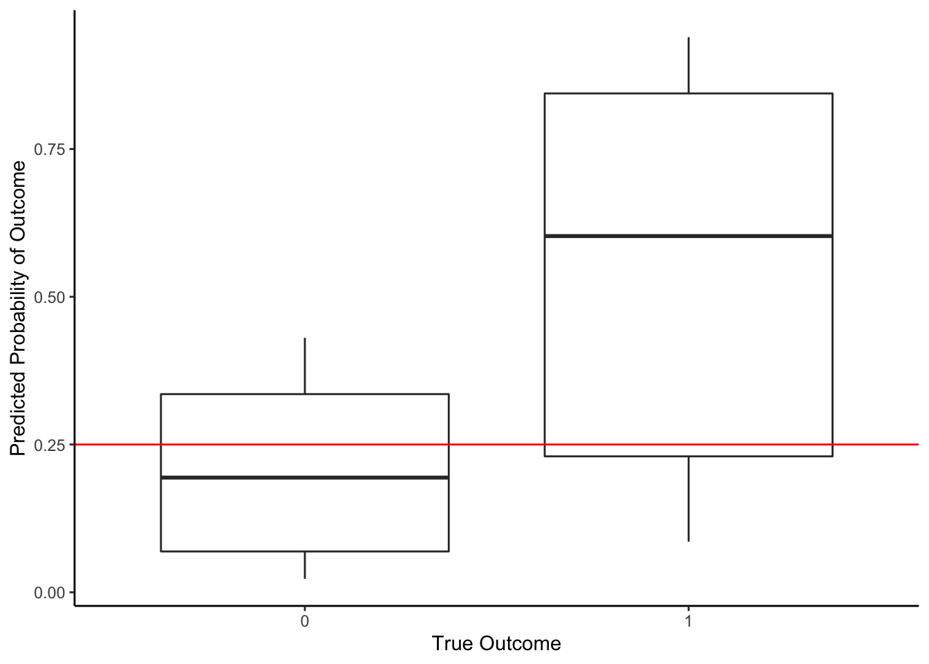
Let’s find our accuracy: (10+4)/(10+3+6+4) = 0.61. Worse than before, but let’s check false negative rate: 3/(3+4) = 0.43. That’s lower. But now we have a non-zero false positive rate: 6/(6+10) = 0.375. So of the experiments with no o-ring failure, we predicted incorrectly 37.5% of the time.
threshold <- 0.25

augment(model.glm, type.predict ='response') %>%
  mutate(predictFail = .fitted >= threshold) %>%
  count(Fail, predictFail) %>%
  mutate(correct = (Fail == predictFail)) %>%
  group_by(Fail) %>%
  mutate(prop = n/sum(n)) #Specificity, False pos, False neg, Sensitivity
## # A tibble: 4 x 5
## # Groups: Fail [2]
## Fail predictFail n correct prop
## <dbl> <lgl> <int> <lgl> <dbl>
## 1 0 FALSE 10 TRUE 0.625
## 2 0 TRUE 6 FALSE 0.375
## 3 1 FALSE 3 FALSE 0.429
## 4 1 TRUE 4 TRUE 0.571Where the threshold goes depends on the real consequences of making those two types of errors and needs to be made in the social and ethical context of the data.