5.3 Simulating Random Sampling from a Population

The data set that we will work with contains ALL flights leaving New York City in 2013. This data represents a full census of the target population of flights leaving NYC in a particular year.

We’ll start by creating two new variables, season defined as winter (Oct - March) or summer (April - Sept) and day_hour defined as morning (midnight to noon) or afternoon (noon to midnight).

data(flights)
flights <- flights %>% 
    na.omit() %>%
    mutate(season = case_when(
      month %in% c(10:12, 1:3) ~ "winter",
      month %in% c(4:9) ~ "summer"
    )) %>% 
    mutate(day_hour = case_when(
      between(hour, 1, 12) ~ "morning",
      between(hour, 13, 24) ~ "afternoon"
    )) %>% 
    select(arr_delay, dep_delay, season, day_hour, origin, carrier)

Since we have the full population of flights in 2013, we could just describe the flights that happened in that year. But, having data on the full population is very rare in practice. Instead, we are going to use this population to illustrate sampling variability.

Let’s take one random sample of 100 flights from the data set, using a simple random sampling strategy.

set.seed(1234) #ensures our random sample is the same every time we run this code
flights_samp1 <- flights %>%
    sample_n(size = 100) ## Sample 100 flights randomly

If you were planning a trip, you may be able to choose between two flights that leave at different times of day. Do morning flights have shorter arrival delays on average than afternoon flights? If so, book the flight earlier in the day!

Let’s look at whether the arrival delay (in minutes) arr_delay differs between the morning and the afternoon, day_hour, by fitting a linear regression model and looking at the estimate for day_hourmorning. This -20.4 minutes is the estimated difference in mean arrival delay times between morning and afternoon flights, so the delay time is less in the morning on average.

flights_samp1 %>%
    with(lm(arr_delay ~ day_hour)) %>%
    tidy()

## # A tibble: 2 x 5
##   term            estimate std.error statistic p.value
##   <chr>              <dbl>     <dbl>     <dbl>   <dbl>
## 1 (Intercept)         14.4      6.38      2.26  0.0258
## 2 day_hourmorning    -20.4     10.6      -1.92  0.0578

At this point, we haven’t looked at the entire population of flights from 2013. Based on one sample of 100 flights, how do you think the time of day impacts arrival delay times in the entire population?

Now, let’s take another random sample of 100 flights from the full population of flights.

flights_samp2 <- flights %>%
    sample_n(size = 100) ## Sample 100 flights randomly

flights_samp2 %>%
    with(lm(arr_delay ~ day_hour)) %>%
    tidy()

## # A tibble: 2 x 5
##   term            estimate std.error statistic p.value
##   <chr>              <dbl>     <dbl>     <dbl>   <dbl>
## 1 (Intercept)         3.15      4.46     0.707   0.481
## 2 day_hourmorning    -2.11      6.44    -0.328   0.744

How does the second sample differ from the first sample? What do they have in common?

We could keep the process going. Take a sample of 100 flights, fit a model, and look at the estimated regression coefficient for day_hourmorning. Repeat many, many times.

We can add a little bit of code to help us simulate this sampling process 1000 times and estimate the difference in mean arrival delay between morning and afternoon for each random sample of 100 flights.

sim_data <- mosaic::do(1000)*( 
    flights %>% 
      sample_n(size = 100) %>%  # Generate samples of 100 flights
      with(lm(arr_delay ~ day_hour)) # Fit linear model
)

Now we have 1000 fit models, each corresponding to one random sample of 100 flights from the population. Let’s summarize and visualize this simulation.

# Summarize
sim_data %>% 
    summarize(
        mean_Intercept = mean(Intercept),
        mean_dayhourmorning = mean(day_hourmorning),
        sd_Intercept = sd(Intercept),
        sd_dayhourmorning = sd(day_hourmorning))

##   mean_Intercept mean_dayhourmorning sd_Intercept sd_dayhourmorning
## 1       13.45053           -14.54158     7.233256           8.87308

# Visualize Intercepts
sim_data %>% 
    ggplot(aes(x = Intercept)) +
    geom_histogram(bins = 15) +
    labs(title = "Sampling distribution of Intercepts\nfrom samples of 100 flights") +
    theme_minimal()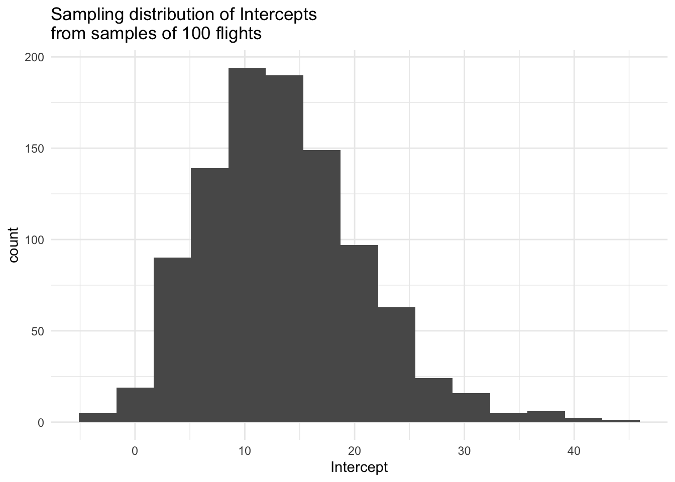

# Visualize Slopes
sim_data %>% 
    ggplot(aes(x = day_hourmorning)) +
    geom_histogram(bins = 15) +
    labs(title = "Sampling distribution of Slopes\nfrom samples of 100 flights") +
    theme_minimal()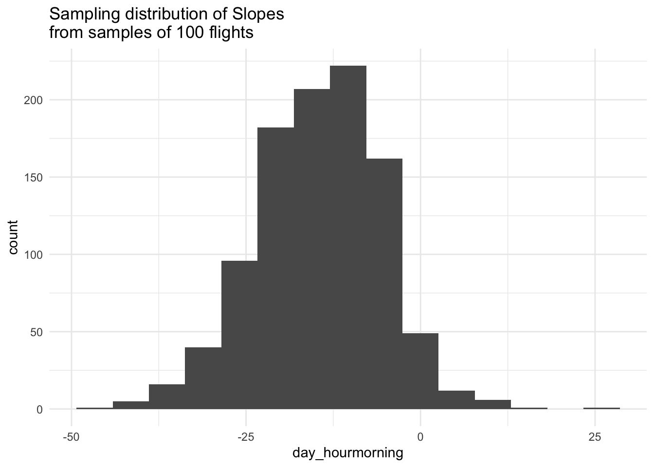

These histograms approximate the sampling distribution of estimated intercepts and the sampling distribution of estimated slopes from a linear model predicting the arrival delay as a function of time of day, both of which describe the variability in the sample statistics across all possible random samples from the population.

Describe the shape, center, and spread of the sampling distribution for the intercepts. Do the same for the slopes.

Notice how these means of the sampling distributions are very close to the population values, below. This makes sense since we are sampling from the population so we’d expect the estimates to bounce around the true population values.

sim_data %>% # Means and standard deviations of sampling distribution
    summarize(
        mean_Intercept = mean(Intercept),
        mean_dayhourmorning = mean(day_hourmorning),
        sd_Intercept = sd(Intercept),
        sd_dayhourmorning = sd(day_hourmorning))

##   mean_Intercept mean_dayhourmorning sd_Intercept sd_dayhourmorning
## 1       13.45053           -14.54158     7.233256           8.87308

flights %>% # Population of flights
    with(lm(arr_delay ~ day_hour)) # Fit linear model

## 
## Call:
## lm(formula = arr_delay ~ day_hour)
## 
## Coefficients:
##     (Intercept)  day_hourmorning  
##           13.42           -14.60