9 Multiple regression principles

Settling In

Sit where you’d like
- Introduce yourself
- Share your names, pronouns, major / minor.
Help each other get ready to take notes!
- Open your notebook. No computer needed today!

We’ll go through the exercises on paper, but the digital version is on the website (qmd here).

Let’s review the Syllabus section about Quizzes & Revisions and Reflections

Recap

Statistical superpowers

The world is full of data!! Thus there are often multiple possible predictors of a response variable Y. Luckily, we can extend a simple linear regression model into a multiple linear regression model:

E[Y | X] = \beta_0 + \beta_1 X_1 + \beta_2 X_2 + \cdots + \beta_1 X_p

Possible benefits:

Descriptive viewpoint: Adding predictors to a model can help us better understand the isolated (causal) effect of a variable by holding constant potential confounders.
Predictive viewpoint: Adding predictors to a model can help us better predict the response variable.

Learning goals

Working with multiple predictors in our plots and models can get complicated!

There are no recipes for this process.

BUT there are some guiding principles that assist in long-term retention, deeper understanding, and the ability to generalize our tools in new settings.

By the end of this lesson, you should be familiar with some general principles for…

incorporating additional quantitative or categorical predictors in a visualization
how additional quantitative or categorical predictors impact the physical representation of a model
interpreting quantitative or categorical coefficients in a multiple regression model

Additional resources

Required:

Multivariate modeling principles (slides)

Extra Examples:

Interpreting multivariate models (Part I) and Part II (slides)

Multiple Linear Regression Principles

Statistical Modeling is as much an Art as a Science

1 Quantitative & 1 Categorical Predictors

Visual: Scatterplot with coloring by group (‘pulling apart’ the categorical groups)
Model: Adding a categorical predictor creates a separate model equation for each group (default: parallel lines)

2 Categorical Predictors

Visual: Side-by-Side Boxplots with coloring by group (‘pulling apart’ the categorical groups)
Model: Adding a categorical predictor creates a separate model equation for each group

2 Quantitative Predictors

Visual: Add another axis or numerical scale (such as color scale)
Model: Adding a quantitative predictor increases physical dimension of model (i.e. creates a 2D plane)

Warm-up

Let’s revisit the bikeshare data:

# Load packages & import data
library(tidyverse)
bikes <- read_csv("https://mac-stat.github.io/data/bikeshare.csv") %>% 
  rename(rides = riders_registered)

Our goal is to explain / predict how registered ridership varies from day to day.

To this end, we’ll build various multiple linear regression models of rides by different combinations of the possible predictors.

# Check out the data
head(bikes)

Example 1: Review visualization

Let’s build a model of rides by windspeed (quantitative) and weekend status (categorical).

bikes %>% 
  select(rides, windspeed, weekend) %>% 
  head()

Write a population model statement for this regression model.
Plot & describe, in words, the relationship between these 3 variables.

# Plot of rides vs windspeed & weekend
# Include a representation of the linear regression model
# HINT: Start with a plot of rides vs windspeed, then add an aesthetic for weekend!

Example 2: Review model

Let’s build the model:

bike_model_1 <- lm(rides ~ windspeed + weekend, data = bikes)
coef(summary(bike_model_1))

The estimated sample model equation is therefore:

E[rides | windspeed, weekendTRUE] = 4738.38 - 63.97 * windspeed - 925.16 * weekendTRUE

This model equation is represented by 2 lines, one corresponding to weekends and the other to weekdays. Simplify the model equation above for weekdays and weekends:

weekdays: rides = ___ - ___ windspeed

weekends: rides = ___ - ___ windspeed

Example 3: Review coefficient interpretation

The intercept coefficient, 4738.38, represents the intercept of the sub-model for weekdays, the reference category. What’s its contextual interpretation?
The windspeed coefficient, -63.97, represents the shared slope of the weekend and weekday sub-models. What’s its contextual interpretation?
The weekendTRUE coefficient, -925.16, represents the change in intercept for the weekend vs weekday sub-model. What’s its contextual interpretation?

Interpreting MLR coefficients (2 predictors)

Consider a multiple linear regression model with 2 predictors:

E[Y | X_1, X_2] = \beta_0 + \beta_1 X_1 + \beta_2 X_2

Then

\beta_0 (“beta 0”) = expected value of Y when X_1 and X_2 are both 0, ie. when all quantitative predictors are set to 0 and the categorical predictors are set to their reference levels.
\beta_1 (“beta 1”) = change in the expected value of Y for two cases whose values of X_1 differ by 1 but who are identical in terms of X_2.
\beta_2 (“beta 2”) = change in the expected value of Y for two cases whose values of X_2 differ by 1 but who are identical in terms of X_1.

Note: If X_j is an indicator variable, then “for two cases whose values of X_j differ by 1” means “comparing the group X_j to the reference level”

Theory Box: Fitting multiple linear regression models

Consider a multiple linear regression model with p predictors:

E[Y|X_1,X_2,...,X_p] = \beta_0 + \beta_1 X_1 + \beta_2 X_2 + ... + \beta_p X_p

We use the least squares criterion to estimate (\beta_0, \beta_1, ..., \beta_p), i.e. we pick the coefficients minimize the sum of squared residuals. Just as with simple linear regression, we can write out a formula for these least square estimates. But for multiple linear regression, this requires linear algebra.

Suppose we have n data points. Using matrix notation, we can collect our observed response values into a vector Y, our predictor values into a matrix X, and our regression coefficients into a vector \beta. The column of 1s in X reflects our model’s inclusion of an intercept:

Y = \left(\begin{array}{c} Y_1 \\ Y_2 \\ \vdots \\ Y_n \end{array} \right) \;\;\;\; \text{ and } \;\;\;\; X = \left(\begin{array}{ccccc} 1 & X_{11} & X_{12} & \cdots & X_{1p} \\ 1 & X_{21} & X_{22} & \cdots & X_{2p} \\ \vdots & \vdots & \vdots & \cdots & \vdots \\ 1 & X_{n1} & X_{n2} & \cdots & X_{np} \\ \end{array} \right) \;\;\;\; \text{ and } \;\;\;\; \beta = \left(\begin{array}{c} \beta_0 \\ \beta_1 \\ \vdots \\ \beta_p \end{array} \right)

Then we can express the model E[Y_i|X_{i1}, X_{i2},...,X_{ip}] = \beta_0 + \beta_1 X_{i1} + \cdots + \beta_p X_{ip} for i \in \{1,...,n\} as:

E[Y|X] = X\beta Further, let \hat{\beta} denote the vector of sample estimated \beta and \hat{Y} denote the vector of predictions / model values:

\hat{Y} = X \hat{\beta}

Thus the sum of squared residuals is

\sum_{i=1}^n (Y_i - \hat{Y}_i)^2 = (Y - \hat{Y})^T(Y - \hat{Y}) = (Y - X \hat{\beta})^T(Y - X \hat{\beta})

and the following formula for sample coefficients \hat{\beta} are the least squares estimates of \beta, i.e. they minimize the sum of squared residuals:

\hat{\beta} = (X^TX)^{-1}X^TY

Exercises

Thus far, we’ve explored a couple examples of multiple regression models that have 2 predictors, 1 quantitative and 1 categorical. Let’s explore what happens when both predictors are categorical or both are quantitative!

Exercise 1: 2 categorical predictors – visualization

Let’s explore the relationship of rides with 2 categorical predictors, weekend status and season.

The below code plots rides vs season.

Modify this code to also include information about weekend.

HINT: Remember the visualization principle that additional categorical predictors require some sort of grouping mechanism / mechanism that distinguishes between the 2 groups.

# rides vs season
bikes %>% 
  ggplot(aes(y = rides, x = season)) + 
  geom_boxplot()

# rides vs season AND weekend
bikes %>%
  ggplot(aes(y = rides, x = season, ___ = ___)) +
  geom_boxplot()

Exercise 2: follow-up

Describe (in words) the relationship of ridership with season & weekend status. In doing so, address the following:

No matter the weekend status, how is ridership associated with season?
No matter the season, how is ridership associated with weekend status?
Does the overall relationship of ridership with season & weekend status appear to be strong?

A model of rides by season alone would be represented by only 4 expected outcomes, 1 for each season. Considering this and the plot above, how do you anticipate a model of rides by season and weekend status will be represented?
- 2 lines, 1 for each weekend status
- 8 lines, 1 for each possible combination of season & weekend
- 2 expected outcomes, 1 for each weekend status
- 8 expected outcomes, 1 for each possible combination of season & weekend

Exercise 3: 2 categorical predictors – build the model

Let’s build the multiple regression model of rides vs season and weekend:

bike_model_2 <- lm(rides ~ weekend + season, bikes)
coef(summary(bike_model_2))

Thus estimated model formula is given by:

E[rides | weekend, season] = 4260.45 - 912.33 weekendTRUE - 116.38 seasonspring + 438.44 seasonsummer - 1719.06 seasonwinter

Use this model to predict the ridership on the following days:

# a fall weekday
4260.45 - 912.33*___ - 116.38*___  + 438.44*___ - 1719.06*___

# a winter weekday    
4260.45 - 912.33*___ - 116.38*___  + 438.44*___ - 1719.06*___

# a fall weekend day        
4260.45 - 912.33*___ - 116.38*___  + 438.44*___ - 1719.06*___

# a winter weekend day
4260.45 - 912.33*___ - 116.38*___  + 438.44*___ - 1719.06*___

Using the calculations in the chunk above, calculate the differences between various predictions:

# diff in predicted ridership on a winter weekday vs a fall weekday
# (that is, the diff btwn 2 days that are at the same time of week but DIFFERENT seasons)
# WHERE HAVE YOU OBSERVED THIS NUMBER BEFORE?!
___ - ___

# diff in predicted ridership on a winter weekend vs a winter weekday
# (that is, the diff btwn 2 days that are in the same season but DIFFERENT times of the week)
# WHERE HAVE YOU OBSERVED THIS NUMBER BEFORE?!
___ - ___

We only made 4 predictions here. How many possible predictions does this model produce? Is this consistent with your intuition in the previous exercise?

Exercise 4: 2 categorical predictors – interpret the model

Use your above predictions and visualization to fill in the below interpretations of the model coefficients.

Hint: What is the consequence of plugging in 0 or 1 for the different weekend and season categories?

Interpreting 4260: On average, we expect there to be 4260 riders on (weekdays/weekends) during the (fall/spring/summer/winter).
Interpreting -912: On average, in any season, we expect there to be 912 (more/fewer) riders on weekends than on ___.
Interpreting -1719: On average, on both weekdays and weekends, we expect there to be 1719 (more/fewer) riders in winter than in ___.

Exercise 5: 2 quantitative predictors – visualization

Next, consider the relationship between rides and 2 quantitative predictors: windspeed and temp_feel. Check out the plot of this relationship below which reflects the visualization principle that quantitative variables require some sort of numerical scaling mechanism – rides and windspeed get numerical axes, and temp_feel gets a color scale:

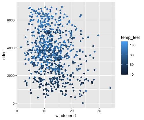
Modify the code below to recreate this plot.

bikes %>%
  ggplot(aes(y = rides, x = windspeed, ___ = ___)) +
  geom_point()

OPTIONAL: Check out this interactive plot which allows us to explore this point cloud in 3D.

library(plotly)
bikes %>% 
  plot_ly(x = ~windspeed, y = ~temp_feel, z = ~rides, 
          type = "scatter3d", 
          mode = "markers",
          marker = list(size = 5, color = ~rides, colorscale = "Viridis"))

Exercise 6: follow-up

Describe (in words) the relationship of ridership with windspeed & temperature. Make sure to comment on all 3 variables, strength of the relationship, and any outliers (if relevant).

Exercise 7: 2 quantitative predictors – modeling

Let’s build the multiple regression model of rides vs windspeed and temp_feel:

bike_model_3 <- lm(rides ~ windspeed + temp_feel, data = bikes)
coef(summary(bike_model_3))

Thus estimated model formula is

E[rides | windspeed, temp_feel] = -24.06 - 36.54 windspeed + 55.52 temp_feel

Interpret the intercept coefficient, -24.06, in context.
Interpret the windspeed coefficient, -36.54, in context.
Interpret the temp_feel coefficient, 55.52, in context.

Exercise 8: Which is “best”?

We’ve now observed 3 different models of ridership, each having 2 predictors. The R-squared values of these models, along with those of the simple linear regression models with each predictor alone, are summarized below.

model	predictors	R-squared
`bike_model_1`	`windspeed` & `weekend`	0.119
`bike_model_2`	`weekend` & `season`	0.349
`bike_model_3`	`windspeed` & `temp_feel`	0.310
`bike_model_4`	`windspeed`	0.047
`bike_model_5`	`temp_feel`	0.296
`bike_model_6`	`weekend`	0.074
`bike_model_7`	`season`	0.279

Which model does the best job of explaining the variability in ridership from day to day?
If you could only pick one predictor, which would it be?
What happens to R-squared when we add a second predictor to our model, and why does this make sense? For example, how does the R-squared for model 1 (with both windspeed and weekend) compare to those of model 4 (only windspeed) and model 6 (only weekend)?
Are 2 predictors always better than 1? Provide evidence and explain why this makes sense.

Exercise 9: Principles of interpretation

These exercises have revealed some principles behind interpreting model coefficients, summarized below.

Review and confirm that these make sense.

Principles of interpretation

Consider a multiple linear regression model:

E[Y | X_1, X_2, ..., X_p] = \beta_0 + \beta_1 X_1 + \beta_2 X_2 + ... + \beta_p X_p

We can interpret the coefficients as follows:

\beta_0 (“beta 0”) is the y-intercept. It describes the average value of Y when X_1, X_2,..., X_p are all 0, ie. when all quantitative predictors are set to 0 and the categorical predictors are set to their reference levels.
\beta_i (“beta i”) is the coefficient of X_i.
- If X_i is quantitative, \beta_i describes the average change in Y associated with a 1-unit increase in X_i while at a fixed set of the other X.
- If X_i represents a category of a categorical variable, \beta_i describes the average difference in Y between this category and the reference category, while at a fixed set of the other X.

Extra practice

Exercise 10: Practice 1

Consider the relationship of rides vs weekend and weather_cat.

Construct a visualization of this relationship.
Construct a model of this relationship.
Interpret the first 3 model coefficients.

Exercise 11: Practice 2

Consider the relationship of rides vs temp_feel and humidity.

Construct a visualization of this relationship.
Construct a model of this relationship.
Interpret the first 3 model coefficients.

Exercise 12: Practice 3

Consider the relationship of rides vs temp_feel and weather_cat.

Construct a visualization of this relationship.
Construct a model of this relationship.
Interpret the first 3 model coefficients.

Exercise 13: CHALLENGE

We’ve explored models with 2 predictors. What about 3 predictors?! Consider the relationship of rides vs temp_feel, humidity, AND weekend.

Construct a visualization of this relationship.
Construct a model of this relationship.
Interpret each model coefficient.

Exercise 14: Explore more examples

Outside of class, check out the below videos that include extra examples:

Interpreting multivariate models (Part I) and Part II (slides)

Wrap Up

Next Monday
- CP 7 (10 minutes before class)
Next Wednesday
- PS 3. Start today!

Solutions

Warm up

Example 1: Review visualization

Solution

bikes %>% 
  ggplot(aes(y = rides, x = windspeed, color = weekend)) + 
  geom_point() + 
  geom_smooth(method = "lm", se = FALSE)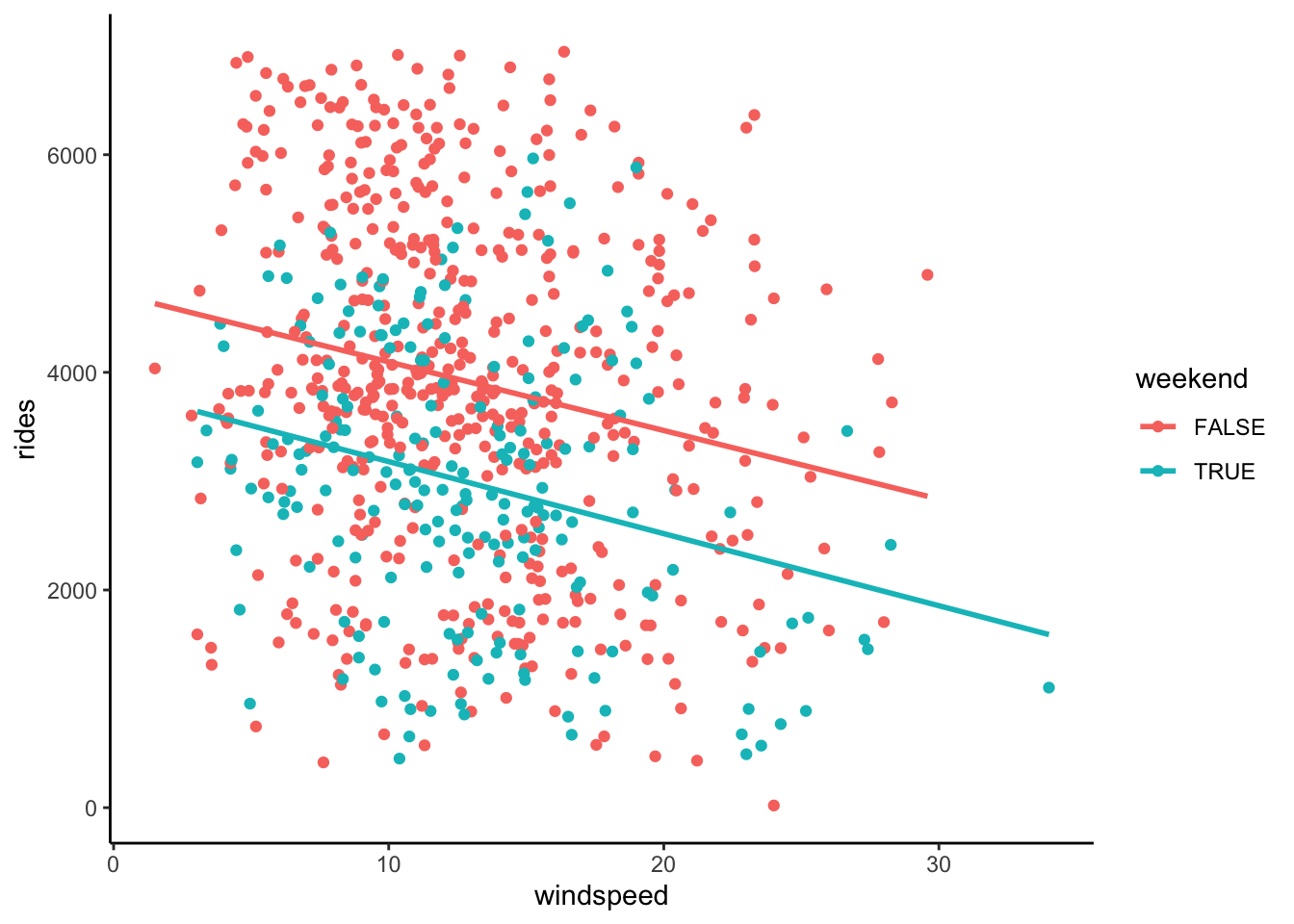

Example 2: Review model

Solution

weekdays: rides = 4738.38 - 63.97 windspeed

weekends: rides = 4738.38 - 63.97 windspeed - 925.16 = 3813.22 - 63.97 windspeed

Example 3: Review coefficient interpretation

Solution

On average, there are 4738 riders on weekdays with 0 windspeed.
On both weekends and weekdays, a 1mph increase in windspeed is associated with 64 fewer riders on average.
At any windspeed, the average ridership is 925 lower on weekends than week days.

Exercises

Exercise 1: 2 categorical predictors – visualization

Solution

bikes %>% 
  ggplot(aes(y = rides, x = season, fill = weekend)) + 
  geom_boxplot()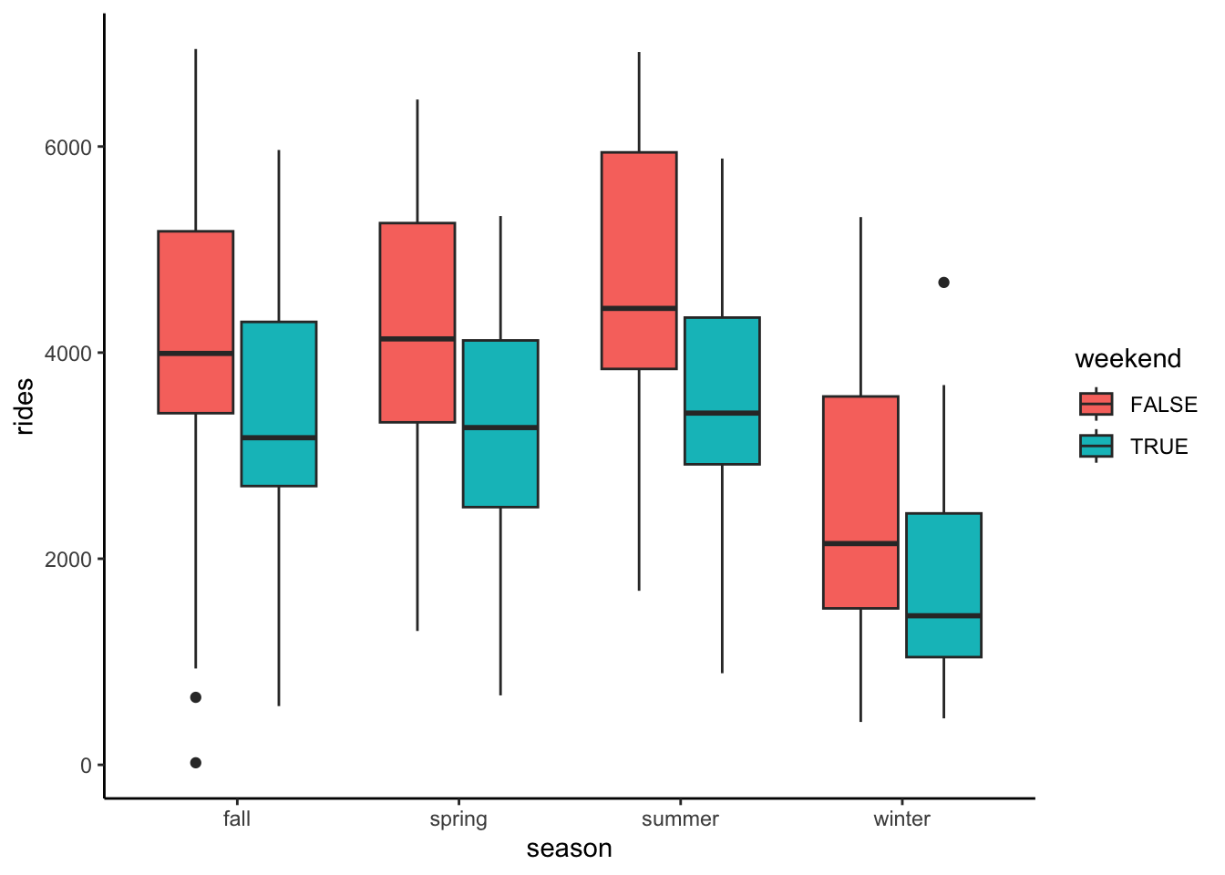

Exercise 2: follow-up

Solution

In every season, ridership tends to be lower on weekends. Across weekend status, ridership tends to be highest in summer and lowest in winter.
8 expected outcomes

Exercise 3: 2 categorical predictors – build the model

Solution

#fall weekday:    
4260.45 - 912.33*0 - 116.38*0 + 438.44*0 - 1719.06*0

[1] 4260.45

#winter weekday:
4260.45 - 912.33*0 - 116.38*0 + 438.44*0 - 1719.06*1

[1] 2541.39

#fall weekend:    
4260.45 - 912.33*1 - 116.38*0 + 438.44*0 - 1719.06*0

[1] 3348.12

#winter weekend:
4260.45 - 912.33*1 - 116.38*0 + 438.44*0 - 1719.06*1

[1] 1629.06

# diff in predicted ridership on a winter weekday vs a fall weekday
# (that is, the diff btwn 2 days that are at the same time of week but DIFFERENT seasons)
# THIS IS THE VALUE OF THE seasonwinter COEF
2541.39 - 4260.45

[1] -1719.06

# diff in predicted ridership on a winter weekend vs a winter weekday
# (that is, the diff btwn 2 days that are in the same season but DIFFERENT times of the week)
# THIS IS THE VALUE OF THE weekendTRUE COEF
1629.06 - 2541.39

[1] -912.33

8: 2 weekend categories * 4 season categories

Exercise 4: 2 categorical predictors – interpret the model

Solution

We expect there to be, on average, 4260 riders on weekdays during the fall.
On average, in any season, there are 912 fewer riders on weekends than on weekdays.
On average, on both weekdays and weekends, we expect there to be 1719 fewer riders in winter than in fall.

Exercise 5: 2 quantitative predictors – visualization

Solution

bikes %>% 
  ggplot(aes(y = rides, x = windspeed, color = temp_feel)) + 
  geom_point()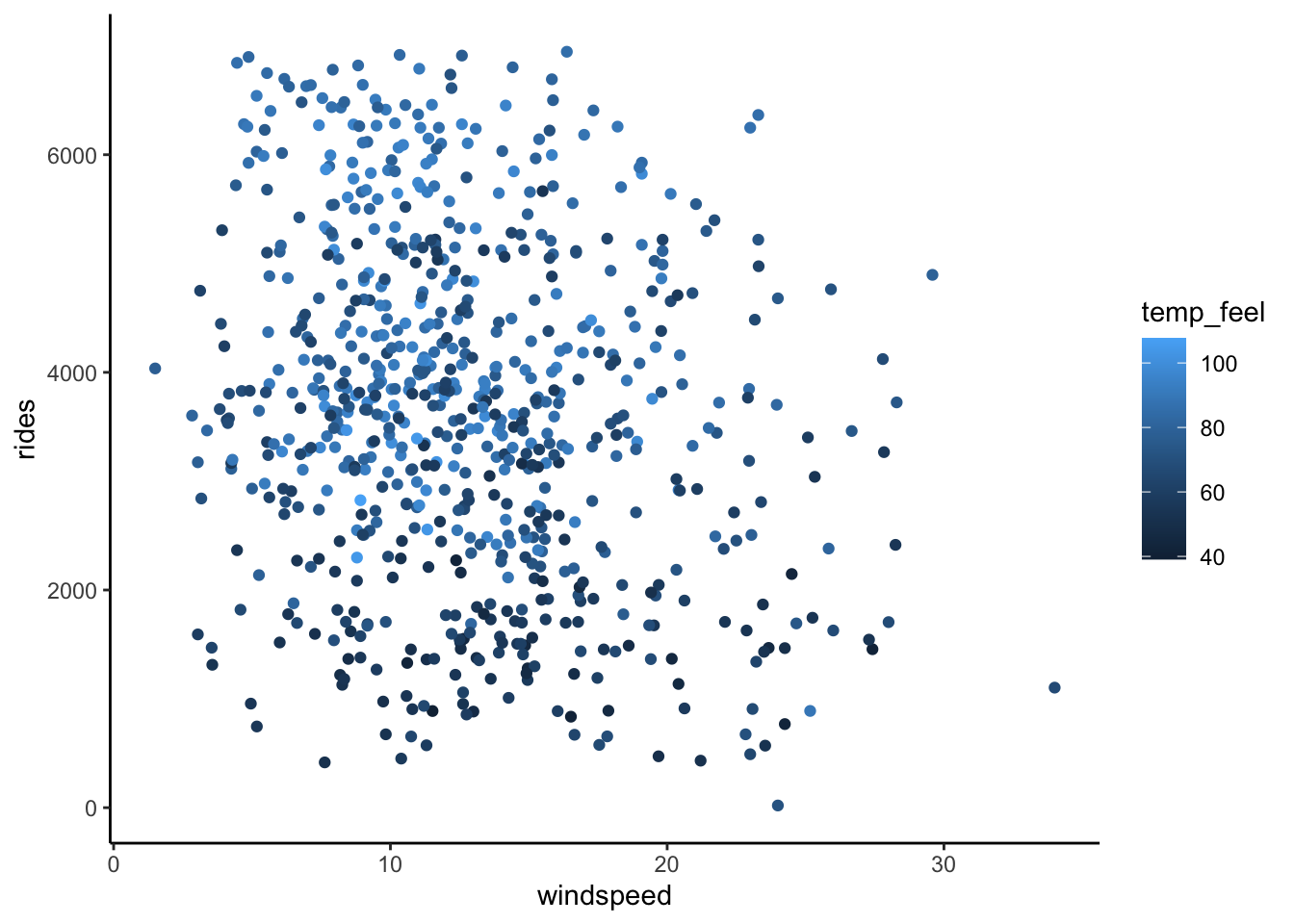

Exercise 6: follow-up

Solution

Ridership tends to increase with temperature (no matter the windspeed) and decrease with windspeed (no matter the temperature).

Exercise 7: 2 quantitative predictors – modeling

Solution

-24.06 = average ridership on days with 0 windspeed and a 0 degree temperature. (Note: this is a correct interpretation, even though it doesn’t make conceptual sense! The model doesn’t know that ridership can’t be negative!)
At any temperature, a 1mph increase in windspeed is associated with a 37 rider decrease in average ridership.
At any windspeed, a 1 degree increase in temperature is associated with a 56 rider increase in average ridership.

Exercise 8: Which is best?

Solution

model 2
temperature
R-squared increases (our model is stronger when we include another predictor)
nope. model 1 (with windspeed and weekend) has a lower R-squared than model 5 (with only temperature)

Exercise 10: Practice 1

Solution

bikes %>% 
  ggplot(aes(y = rides, x = weekend, fill = weather_cat)) + 
  geom_boxplot()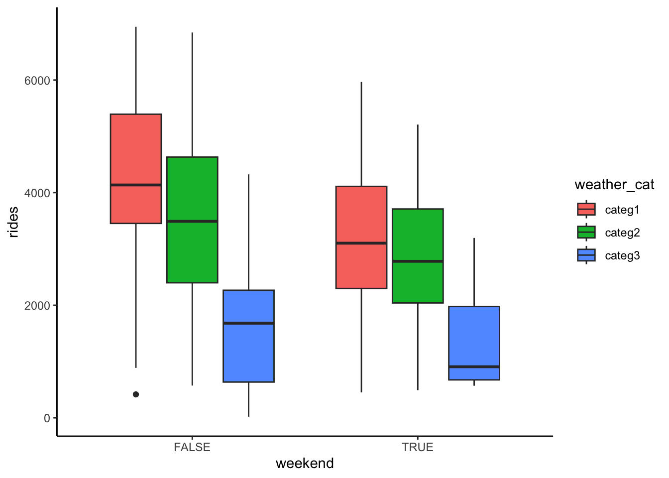

new_model_1 <- lm(rides ~ weekend + weather_cat, bikes)
coef(summary(new_model_1))

                    Estimate Std. Error   t value      Pr(>|t|)
(Intercept)        4211.8741   75.54724 55.751529 9.461947e-265
weekendTRUE        -982.2106  117.24719 -8.377264  2.786301e-16
weather_catcateg2  -608.8640  113.00211 -5.388077  9.628947e-08
weather_catcateg3 -2360.2049  319.71640 -7.382183  4.270163e-13

The average ridership on a weekday with nice weather (categ1) is 4212 rides.
On days with the same weather, the average ridership is 982 less on a weekend than on a weekday.
On any day of the week, the average ridership is 609 less on dreary days than on nice days.

Exercise 11: Practice 2

Solution

bikes %>% 
  ggplot(aes(y = rides, x = temp_feel, color = humidity)) + 
    geom_point()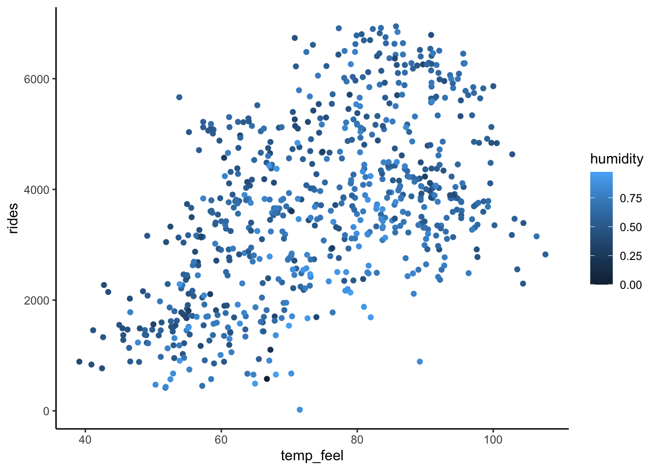

new_model_2 <- lm(rides ~ temp_feel + humidity, bikes)
coef(summary(new_model_2))

               Estimate Std. Error   t value     Pr(>|t|)
(Intercept)   315.83704 303.777334  1.039699 2.988249e-01
temp_feel      60.43316   3.272315 18.468015 9.451345e-63
humidity    -1868.99356 336.963661 -5.546573 4.078901e-08

On average, there are 316 riders on days with 0 humidity that feel like 0 degrees.
At any humidity, a 1 degree increase in ridership is associated with a 60 ride increase in average ridership.
At any temperature, a 1 percentage point increase in humidity (i.e. a 0.1 increase in humidity) is associated with a 187 decrease in average ridership.

Exercise 12: Practice 3

Solution

new_model_3 <- lm(rides ~ temp_feel + weather_cat, bikes)
coef(summary(new_model_3))

                     Estimate Std. Error   t value     Pr(>|t|)
(Intercept)        -288.68840 251.264383 -1.148943 2.509574e-01
temp_feel            55.30133   3.215495 17.198387 7.082670e-56
weather_catcateg2  -386.42241 100.187725 -3.856984 1.249775e-04
weather_catcateg3 -1919.01375 283.022420 -6.780430 2.481218e-11

bikes %>% 
  ggplot(aes(y = rides, x = temp_feel, color = weather_cat)) + 
  geom_point() + 
  geom_line(aes(y = new_model_3$fitted.values), size = 1.5)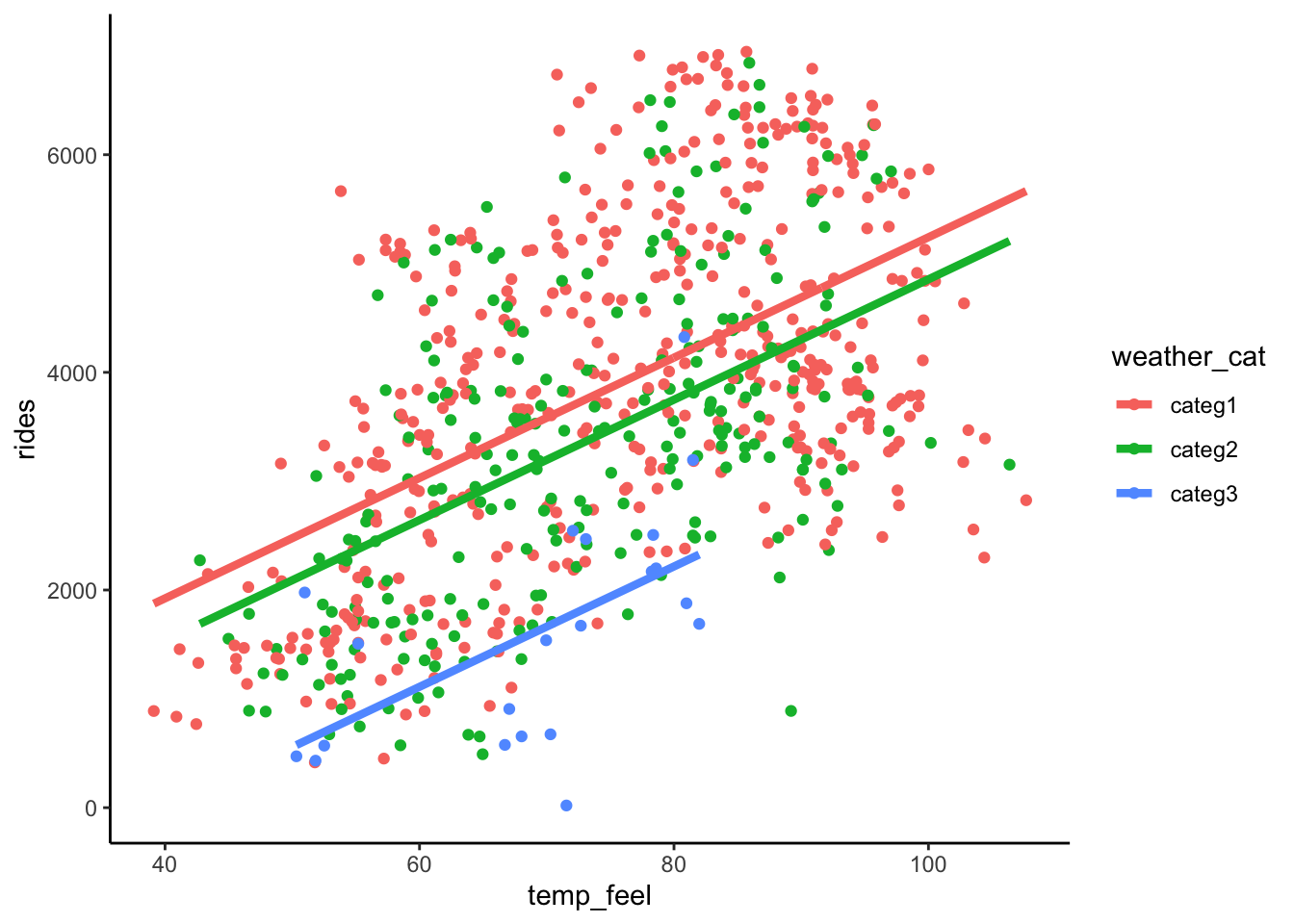

On average, there are -289 riders on nice weather days that feel like 0 degrees. (Note: this is a correct interpretation, even though it doesn’t make conceptual sense!)
On days with the same weather, a 1 degree increase in temperature is associated with a 55 ride increase in average ridership.
On days with the same temperature, average ridership is 386 rides lower on a dreary weather day than on a nice weather day.

Exercise 13: CHALLENGE

Solution

bikes %>% 
  ggplot(aes(y = rides, x = temp_feel, color = humidity, size = weekend)) + 
  geom_point()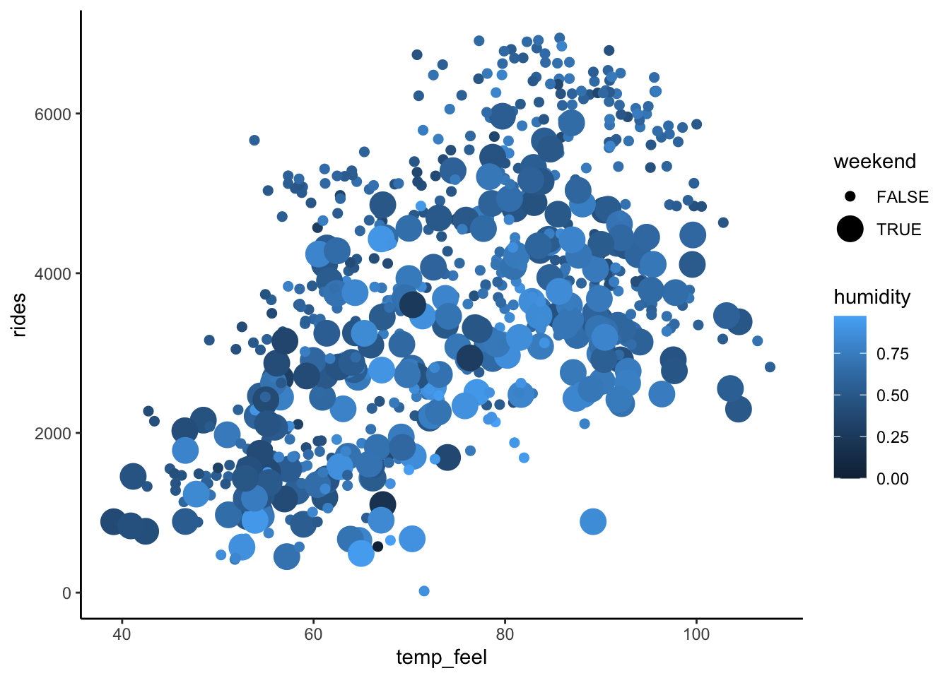

new_model_4 <- lm(rides ~ temp_feel + humidity + weekend, bikes)
coef(summary(new_model_4))

               Estimate Std. Error   t value     Pr(>|t|)
(Intercept)   668.60236 292.181063  2.288315 2.240530e-02
temp_feel      59.36751   3.119256 19.032585 7.626695e-66
humidity    -1906.43437 320.982938 -5.939364 4.433789e-09
weekendTRUE  -869.05771 100.057822 -8.685555 2.471050e-17

On average, there are 669 riders on weekdays that feel like 0 degrees and have no humidity.
On days with the same humidity levels and time of the week, a 1 degree increase in temperature is associated with a 59 ride increase in average ridership.
On days with the same temperature and time of the week, a 0.1 point increase in humidity levels (i.e. a 1 percentage point increase in humidity) is associated with a 190.6 ride decrease in average ridership.
On days with the same temperature and humidity, the average ridership is 869 rides lower on weekends compared to weekdays.