# Load the data & packages
library(tidyverse)
fish <- read_csv("https://Mac-STAT.github.io/data/Mercury.csv")20 Sampling distributions, the CLT, and Bootstrapping
Settling In
- Take 5 minutes to jot down thoughts/ideas for your Midsemester 2 Reflection (due on Friday)
- Find your individual Google doc (link in a recent email from Prof. Heggeseth)
- Find the qmd here: “20-sampling-dist-clt-bootstrap-notes.qmd”.
Recap
ImportantStatistical superpowers
In order to use our sample data to make inferences about the broader population from which we took the sample, we need a sense of the potential error in our sample estimates.
Though it’s impossible to know exactly how far off our estimates are from the actual population parameters (since we don’t know the value of those parameters), we can apply both theory and simulation to our sample in order to inform our understanding.
NoteLearning goals
Let \beta be some population parameter and \hat{\beta} be a sample estimate of \beta. Our goals for the day are to:
- use simulation to solidify our understanding of sampling distributions and standard errors
- explore and compare two approaches to approximating the sampling distribution of \hat{\beta}:
- Central Limit Theorem (CLT)
- bootstrapping
- explore the impact of sample size on sampling distributions and standard errors
NoteAdditional resources
Required:
- Reading: Section 6.7 in the STAT 155 Notes
- Video 1: sampling distributions
- Video 2: Central Limit Theorem
- Video 3: bootstrapping
Sampling Distribution
A sampling distribution gives the values and plausibility of values of sample estimates across all possible samples from the same population of a given sample size n.
How much these estimates vary across possible samples is measured by the standard error.

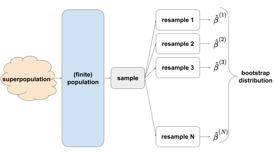
Here are terms related to the image above:
Superpopulation: The true underlying process that governs the relationships of interest.
Finite Population: At the time the data was collected, the possible observable cases in the larger population and the relationships of interest in that population at that time.
Sample: In our data, the observed, recorded cases and the estimated relationships amongst them.
- In last class, we simulated the sampling distribution by having each person take a sample from the same “known” population of movies.
- In practice, we only have 1 sample from the population.
There are two main ways of approximating the sampling distribution,
- central limit theorem (CLT), a theory-based approach
- bootstrapping, a computing-based approach
Central Limit Theorem
When our sample size n is “large enough”, we can approximate the sampling distribution using the CLT (a mathematical theorem):
\hat{\beta}_j \sim N(\beta_j, \text{ standard error}^2)
Sampling Distribution of \hat{\beta}_j
- Shape: Unimodal, symmetric (68-95-99.7 Rule)
- Center: mean of sampling distribution is the true unknown population parameter
- Spread: sd of sampling distribution is the standard error
Bootstrapping
Treat sample as a “fake population” and simulate by sampling WITH replacement
- each simulated sample is of size n, the same size as the original sample
- calculate estimate within each simulated sample (“resample”)
- create many (~500) simulated samples and thus samples estimates
Sampling Distribution of \hat{\beta}_j
- Shape observed through density plot (often approx. unimodal, symmetric)
- Center at original sample estimate, calculating the mean across simulated samples
- Spread by calculating the standard deviation across simulated samples (standard error)
Warm-Up
Rivers contain small concentrations of mercury which can accumulate in fish. Scientists studied this phenomenon among largemouth bass in the Wacamaw and Lumber rivers of North Carolina.
One goal of this study was to explore the relationship of a fish’s mercury concentration (Concen) with its size, specifically its Length:
E(Concen | Length) = \beta_0 + \beta_1 Length
To estimate this relationship, they caught and evaluated 171 fish, and recorded the following:
| variable | meaning |
|---|---|
| River | Lumber or Wacamaw |
| Station | Station number where the fish was caught (0, 1, …, 15) |
| Length | Fish’s length (in centimeters) |
| Weight | Fish’s weight (in grams) |
| Concen | Fish’s mercury concentration (in parts per million; ppm) |
Example 1: Population parameter vs sample estimate
Plot and model the relationship of mercury concentration with length:
fish %>%
  ggplot(aes(y = Concen, x = Length)) +
  geom_point() +
  geom_smooth(method = "lm", se = FALSE)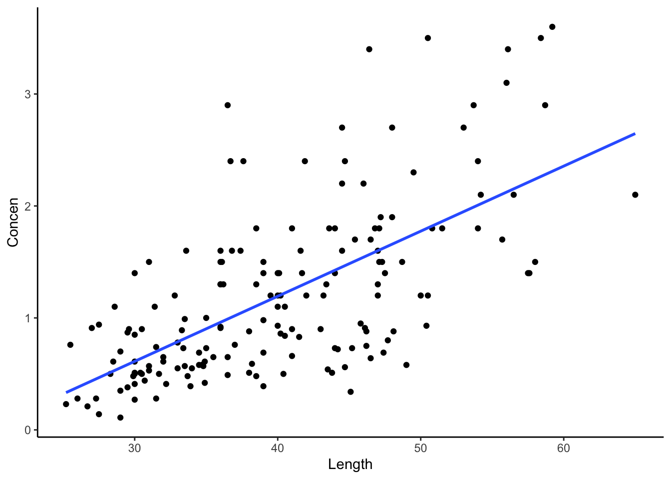
fish_model <- lm(Concen ~ Length, data = fish)
coef(summary(fish_model))
Estimate Std. Error t value Pr(>|t|)
(Intercept) -1.13164542 0.213614796 -5.297598 3.617750e-07
Length 0.05812749 0.005227593 11.119359 6.641225e-22In the summary table, is the Length coefficient 0.058 the population parameter \beta_1 or a sample estimate \hat{\beta}_1?
Example 2: Sampling distributions
Since we don’t know \beta_1, we can’t know the exact error in \hat{\beta}_1! This is where sampling distributions come in.
They describe how estimates \hat{\beta}_1 might vary from sample to sample, thus how far these estimates might fall from \beta_1 (i.e. the standard error):
For each of the concepts in the diagram above (Superpopulation, Finite Population, Sample), these represent for this specific data example:
Superpopulation: The true underlying process that governs the relationship between mercury concentration and length of fish, for every fish that has ever existed and ever will exist in these two rivers!
Finite Population: At the time the data was collected, the true observed relationship between mercury concentration and length of fish, for all fish in the two rivers at that time.
Sample: In our data, the observed/estimated relationship between mercury concentration and length of fish (this is \hat{\beta}_1!).
Example 3: Approximating the sampling distribution
In practice, we only take 1 sample of data (e.g. 1 sample of 171 fish). We can’t go out and take every possible sample of 171 fish!
- Thus we don’t have access to the sampling distribution…
- Thus we don’t actually know the standard error of the sample estimates…
- Thus we need to approximate the sampling distribution / standard error using our 1 sample.
We’ll take 2 different approaches:
- Central Limit Theorem (CLT) (theory / formula-based approach)
When our sample size n is “large enough”, we might approximate the sampling distribution using the CLT:
\hat{\beta}_1 \sim N(\beta_1, \text{ standard error}^2)
The standard error in the CLT is approximated from our sample via some formula c / \sqrt{n} where “c” is complicated. It’s reported in a model summary() table!
- Bootstrapping (simulation approach)
In practice, we can’t simulate the sampling distribution by repeatedly taking samples from the population – we only take 1 sample of size n!!
But we can REsample our sample:
- we sample our sample WITH replacement (you’ll explore why below)
- each REsample is of size n, the same size as the original sample (so that we can assess the potential error associated with samples the same size as ours)
This helps us approximate the shape of the sampling distribution and the standard error of our estimate:
If it feels somewhat magical to you that this works out, that’s a very reasonable feeling.
The saying “to pull oneself up by the bootstraps” is often attributed to Rudolf Erich Raspe’s 1781 The Surprising Adventures of Baron Munchausen in which the character pulls himself out of a swamp by his hair (not bootstraps). In short, it means to get something from nothing, through your own effort:

In this spirit, statistical bootstrapping doesn’t make any probability model assumptions. It uses only the information from our one sample to approximate standard errors.
REFLECT: Approximating the sampling distribution – CLT vs Bootstrapping
Great! We have two options. Here are some things to think about / reflect on:
- CLT
- The quality of this approximation hinges upon the validity of the Central Limit Theorem which hinges upon the validity of the theoretical model assumptions, as well as a “large enough” sample size n.
- The CLT uses theoretical formulas for the standard error estimates, thus can feel a little mysterious without a solid foundation in probability theory.
- BUT: When the theory is “valid”, nothing beats a CLT approximation!!!
- Bootstrapping
- The statistical theory behind bootstrapping is quite complicated, and there are certain obscure cases (none that we will encounter in STAT 155) where the assumptions underlying bootstrapping fail to hold.
- It cannot and should not replace the CLT. BUT, it but gives us some nice intuition behind the idea of resampling, which is fundamental for hypothesis testing (which we’ll get to shortly!).
Reflect: Before testing them out, what questions do you have about either approach? What do you think would help you build more intuition for the CLT and/or bootstrapping? Does one approach resonate with you more than the other?
Exercises
Goals:
- Learn how to implement the bootstrapping technique.
- Use bootstrapping to explore the impact of sample size on standard errors, and the sampling distribution more generally.
- Compare bootstrapping and CLT approximations.
Exercise 1: Why “resampling” (replace = TRUE)?
Recall that in bootstrapping, we REsample our sample – we sample it with replacement. Let’s wrap our minds around this idea using a small example of just the first 4 fish in our data:
small_sample <- fish %>%
  select(Concen, Length) %>%
  head(4)

small_sample
This sample produces an estimated Length coefficient of 0.06532:
lm(Concen ~ Length, data = small_sample)- The chunk below samples 4 fish without replacement from our
small_sampleof 4 fish. Run it several times, then discuss:
- What do you observe about the samples themselves?
- If we used each one of these samples to estimate the model of
ConcenbyLength, what do you anticipate will happen?
small_sample %>%
sample_n(size = 4, replace = FALSE)- Test your intuition. The chunk below samples 4 fish from the
small_samplewithout replacement (replace = FALSE), then uses it to estimate the model ofConcenbyLength. Run it several times, then discuss:
- What do you observe about the sample models?
- What’s the problem with this?
small_sample %>%
  sample_n(size = 4, replace = FALSE) %>%
with(lm(Concen ~ Length))- Sampling our sample without replacement merely returns our original sample, thus does NOT give us any sense of sampling variability! Instead, REsample 4 fish from our
small_samplewith replacement. Run it several times. What do you notice about the samples themselves?
small_sample %>%
  sample_n(size = 4, replace = TRUE)
Similarly, what do you notice about the sample models built from the REsamples?
small_sample %>%
  sample_n(size = 4, replace = TRUE) %>%
  with(lm(Concen ~ Length))
NoteReflect: Resampling
REsampling our sample provides insight into sampling variability, hence potential error in our sample estimates. Each REsample might include some original sample subjects several times, and others not at all. But this is a good thing!
- Observing a subject multiple times in a REsample mimics the idea that there are several separate but similar subjects in the population!
- Sampling with replacement ensures that our resampled observations are independent, which we need in order for bootstrapping to “work”!
Exercise 2: Run a bootstrap simulation
Recall that we can sample, say, 10 observations from our dataset with replacement using sample_n():
# Run this chunk a few times to explore the different samples you get
fish %>%
  sample_n(size = 10, replace = TRUE)
We can also take a sample and then use the data to estimate the model:
# Run this chunk a few times to explore the different sample models you get
fish %>%
  sample_n(size = 10, replace = TRUE) %>%
  with(lm(Concen ~ Length))
We can also take multiple unique samples and build a sample model from each.
The code below obtains 500 separate samples of 10 fish, and stores the model estimates from each:
# Set the seed so that we all get the same results
set.seed(155)

# Store the sample models
sample_models_10 <- map_df(1:500, function(i){
    fish %>%
    sample_n(size = 10, replace = TRUE) %>%
    lm(Concen ~ Length, data = .) %>%
    coef()
})


# Check it out
head(sample_models_10)
dim(sample_models_10)
What’s the point of the
map_df()function?!? If you’ve taken any COMP classes, what process do you thinkmap_df()is a shortcut for?What is stored in the
InterceptandLengthcolumns of the results?We’ll obtain a bootstrapping distribution of \hat{\beta}_1 by taking many (500, in this case) different REsamples and exploring the degree to which \hat{\beta}_1 varies from sample to sample. REMEMBER: Each bootstrap resample must be the same size as our original dataset: 171 fish (not 10). Why? We’re trying to understand the potential error in using our sample of 171 fish, not 10 fish!
Edit the code below to obtain a bootstrapping distribution.
# Set the seed so that we all get the same results
set.seed(155)

# Store the sample models
sample_models_boot <- map_df(1:___, function(i){
    fish %>%
    sample_n(size = ___, replace = TRUE) %>%
    lm(Concen ~ Length, data = .) %>%
    coef()
})
Exercise 3: Bootstrap distribution & standard error
Check out the resulting 500 bootstrapped sample models. The red line represents the model estimate calculated from our original sample of 171 fish (not the population model, which we don’t know!):
fish %>%
  ggplot(aes(x = Length, y = Concen)) +
  geom_smooth(method = "lm", se = FALSE) +
  geom_abline(data = sample_models_boot,
              aes(intercept = `(Intercept)`, slope = Length),
              color = "gray", size = 0.25) +
  geom_smooth(method = "lm", color = "red", se = FALSE)
Let’s focus on the slopes of these 500 sample models.
A plot of the 500 slopes approximates features of the sampling distribution of the sample slopes.
sample_models_boot %>%
  ggplot(aes(x = Length)) +
  geom_density() +
  geom_vline(xintercept = 0.05813, color = "red")
Describe the sampling distribution:
What’s its general shape?
Where is it roughly centered? Is this value the “true” population slope \beta_1 or our sample slope estimate \hat{\beta}_1?
Roughly what’s its spread / i.e. what’s the range of estimates you observed?
For a more rigorous assessment of the spread among the bootstrap slopes, calculate their standard deviation. This provides a bootstrap approximation of the standard error of the slope estimates. IMPORTANT RECALL: The standard error measures the typical distance of a sample estimate from the actual population value. Approximating the standard error, hence understanding the potential error in our sample estimate, is a key goal here!
sample_models_boot %>%
  ___(sd(Length))
Exercise 4: CLT distribution & standard error
Recall that the CLT provides a formula / theory-based alternative to approximating features of the sampling distribution. It assumes that, so long as our sample size is “big enough”, the sampling distribution of the sample slope \hat{\beta}_1 will be Normally distributed around the population slope \beta_1 with some standard error:
\hat{\beta}_1 \sim N(\beta_1, \text{ standard error}^2)
The CLT-related approximation of the standard error of the slope estimates is calculated via a complicated formula, not simulation. This is reported in the model summary() table, in the Std. Error column.
coef(summary(fish_model))Is the CLT assumption of Normality consistent with the shape of the bootstrapping distribution in the previous exercise?
Are the CLT and bootstrap estimates of the standard error roughly equivalent?
Want more intuition into the CLT? Watch this video explanation using bunnies and dragons: https://www.youtube.com/watch?v=jvoxEYmQHNM
Exercise 5: Using the CLT
Plugging in the estimated standard error of 0.005, the complete CLT approximation of the sampling distribution of \hat{\beta}_1 is:
\hat{\beta}_1 \sim N(\beta_1, 0.005^2) Use this result with the 68-95-99.7 property of the Normal model to understand the potential error in a slope estimate.
a. There are many possible samples of 171 fish. What percent of these will produce an estimate \hat{\beta}_1 that’s within 0.010, i.e. 2 standard errors, of the actual population slope \beta_1?
More than 2 standard errors from \beta_1?
More than 0.015, i.e. 3 standard errors, above \beta_1?
Exercise 6: CLT and the 68-95-99.7 Rule
Fill in the blanks below to complete some general properties assumed by the CLT:
___% of samples will produce \hat{\beta}_1 estimates within 1 st. err. of \beta_1
___% of samples will produce \hat{\beta}_1 estimates within 2 st. err. of \beta_1
___% of samples will produce \hat{\beta}_1 estimates within 3 st. err. of \beta_1
Exercise 7: Increasing sample size
Now that we trust bootstrapping simulations to provide reasonable insight into sampling distributions (they agree with the CLT!), let’s use them to explore the impact of sample size on the quality of our sample estimates. Recall our different (bootstrap) sample estimates when we started with a sample of 171 fish:
# All bootstrap sample models
fish %>%
  ggplot(aes(x = Length, y = Concen)) +
  geom_smooth(method = "lm", se = FALSE) +
  geom_abline(data = sample_models_boot,
              aes(intercept = Intercept, slope = Length),
              color = "gray", size = 0.25)
# Slopes of all bootstrap sample models
sample_models_boot %>%
ggplot(aes(x = Length)) +
geom_density()Suppose that instead of starting with n = 171 fish, we only had a sample of n = 50 or n = 20 fish! What impact do you anticipate this having on our sample estimates:
If we had a smaller sample, how would it impact the sample model lines (top plot): Do you expect there to be more or less variability among the sample model lines?
If we had a smaller sample, how would it impact the sampling distribution of the sample slopes (bottom plot):
- Around what value to you expect it be centered?
- What general shape do you expect it to have?
- Do you expect it to be narrower (with smaller standard error) or wider (with larger standard error)?
Exercise 8: 500 samples of size n
Let’s decrease the sample size in our simulation. First, take 500 REsamples from fish, but this time make each resample just 50 fish. Then build a sample model from each sample:
set.seed(155)
sample_models_50 <- map_df(1:500, function(i){
    fish %>%
    sample_n(size = ___, replace = TRUE) %>%
    ___(Concen ~ Length, data = .) %>%
    ___()
})


# Check it out
# Make sure that your first Intercept estimate is -1.9990216
head(sample_models_50)
Similarly, take 500 REsamples of size 20 from fish, then build a sample model from each sample:
set.seed(155)
sample_models_20 <- map_df(1:500, function(i){
    fish %>%
    sample_n(size = ___, replace = TRUE) %>%
    ___(Concen ~ Length, data = .) %>%
    ___()
})

# Check it out
# Make sure that your first Intercept estimate is -2.2383596
head(sample_models_20)
Exercise 9: Impact of sample size (part I)
Use the 3 plots below to compare and contrast the 500 sets of sample models when using samples of size 20, 50, and 171. What happens as we increase sample size?! Was this what you expected?
# 500 sample models using samples of size 20
fish %>%
  ggplot(aes(x = Length, y = Concen)) +
  geom_smooth(method = "lm", se = FALSE) +
  geom_abline(data = sample_models_20,
              aes(intercept = `(Intercept)`, slope = Length),
              color = "gray", size = 0.25) +
  lims(x = c(25, 65), y = c(-1, 5))
# 500 sample models using samples of size 50
fish %>%
ggplot(aes(x = Length, y = Concen)) +
geom_smooth(method = "lm", se = FALSE) +
geom_abline(data = sample_models_50,
aes(intercept = `(Intercept)`, slope = Length),
color = "gray", size = 0.25) +
lims(x = c(25, 65), y = c(-1, 5))# 500 sample models using samples of size 171
fish %>%
ggplot(aes(x = Length, y = Concen)) +
geom_smooth(method = "lm", se = FALSE) +
geom_abline(data = sample_models_boot,
aes(intercept = `(Intercept)`, slope = Length),
color = "gray", size = 0.25) +
lims(x = c(25, 65), y = c(-1, 5))Exercise 10: Impact of sample size (part II)
Using the 3 plots below, let’s focus on just the sampling distributions of our 500 slope estimates \hat{\beta}_1, i.e. the slopes of the lines in the above plots. How do the shapes, centers, and spreads of these sampling distributions compare? Was this what you expected?
# 500 sample slopes using samples of size 20
sample_models_20 %>%
ggplot(aes(x = Length)) +
geom_density() +
lims(x = c(-0.01, 0.13), y = c(0, 70))# 500 sample slopes using samples of size 50
sample_models_50 %>%
ggplot(aes(x = Length)) +
geom_density() +
lims(x = c(-0.01, 0.13), y = c(0, 70))# 500 sample slopes using samples of size 171
sample_models_boot %>%
ggplot(aes(x = Length)) +
geom_density() +
lims(x = c(-0.01, 0.13), y = c(0, 70))Exercise 11: Properties of sampling distributions
In light of your observations, complete the following statements about the sampling distribution of the sample slope.
For all sample sizes, the shape of the sampling distribution is roughly ___ and the sampling distribution is roughly centered around ___, the sample estimate from our original data.
As sample size increases:
The average sample slope estimate INCREASES / DECREASES / IS FAIRLY STABLE.
The standard error of the sample slopes INCREASES / DECREASES / IS FAIRLY STABLE.Thus, as sample size increases, our sample slopes become MORE RELIABLE / LESS RELIABLE.
Wrap-up
- Finish and study the activity!
- No Class Friday (work on Project Milestone 1 - qmd in Moodle)
- Project Milestone 1 (individual) due April 6
- Midsemester 2 Reflection due Friday
Solutions
Warm-up
Example 1: Population parameter vs sample estimate
Solution
This is \hat{\beta}_1, a sample estimate of the population parameter \beta_1.
Exercises
Exercise 1: Why “resampling” (replace = TRUE)?
Solution
small_sample <- fish %>%
select(Concen, Length) %>%
head(4)
small_sample# A tibble: 4 × 2
Concen Length
<dbl> <dbl>
1 1.6 47
2 1.5 48.7
3 1.7 55.7
4 0.73 45.2lm(Concen ~ Length, data = small_sample)
Call:
lm(formula = Concen ~ Length, data = small_sample)
Coefficients:
(Intercept) Length
-1.82781 0.06532 - These samples always have the same 4 fish, just in different orders.
- Intuition
small_sample %>%
sample_n(size = 4, replace = FALSE)# A tibble: 4 × 2
Concen Length
<dbl> <dbl>
1 0.73 45.2
2 1.5 48.7
3 1.6 47
4 1.7 55.7- Since the samples are the same, the sample models are always the same
- This doesn’t provide insight into how our results can vary from sample to sample
small_sample %>%
sample_n(size = 4, replace = FALSE) %>%
with(lm(Concen ~ Length))
Call:
lm(formula = Concen ~ Length)
Coefficients:
(Intercept) Length
-1.82781 0.06532 - We sometimes get the same fish more than once!
set.seed(1)small_sample %>%
sample_n(size = 4, replace = TRUE)# A tibble: 4 × 2
Concen Length
<dbl> <dbl>
1 0.73 45.2
2 0.73 45.2
3 1.6 47
4 0.73 45.2The sample models can differ!
small_sample %>%
sample_n(size = 4, replace = TRUE) %>%
with(lm(Concen ~ Length))
Call:
lm(formula = Concen ~ Length)
Coefficients:
(Intercept) Length
-1.82781 0.06532 Exercise 2: Run a bootstrap simulation
Solution
map_df()repeats the code within the parentheses as many times as you tell it. map_df()` does repetition like a for loop.500 different sample estimates of the model
# Set the seed so that we all get the same results
set.seed(155)
# Store the sample models
sample_models_boot <- map_df(1:500, function(i){
fish %>%
sample_n(size = 171, replace = TRUE) %>%
lm(Concen ~ Length, data = .) %>%
coef()
})Exercise 3: Bootstrap distribution & standard error
Solution
fish %>%
ggplot(aes(x = Length, y = Concen)) +
geom_smooth(method = "lm", se = FALSE) +
geom_abline(data = sample_models_boot,
aes(intercept = `(Intercept)`, slope = Length),
color = "gray", size = 0.25) +
geom_smooth(method = "lm", color = "red", se = FALSE)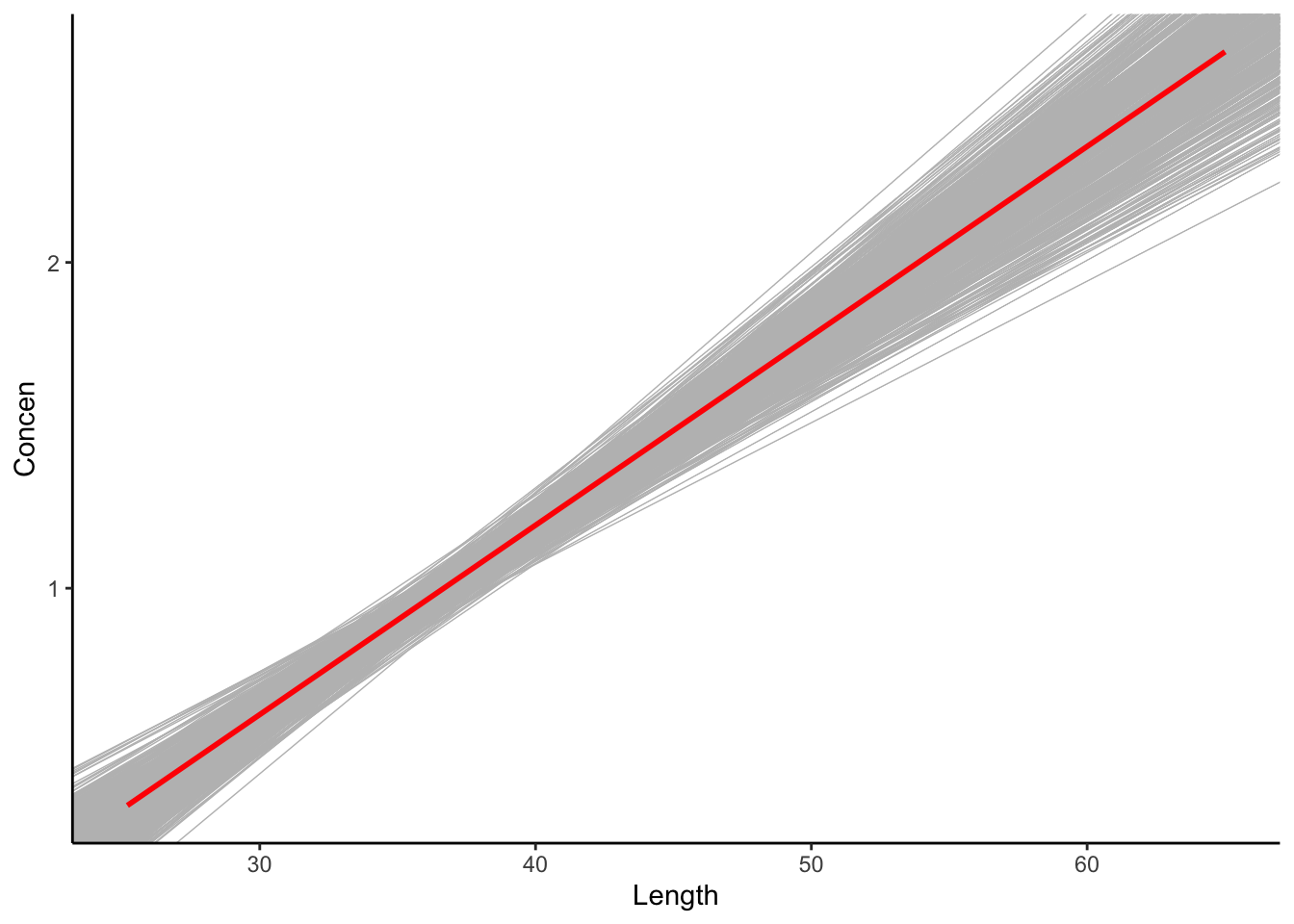
sample_models_boot %>%
ggplot(aes(x = Length)) +
geom_density() +
geom_vline(xintercept = 0.05813, color = "red") 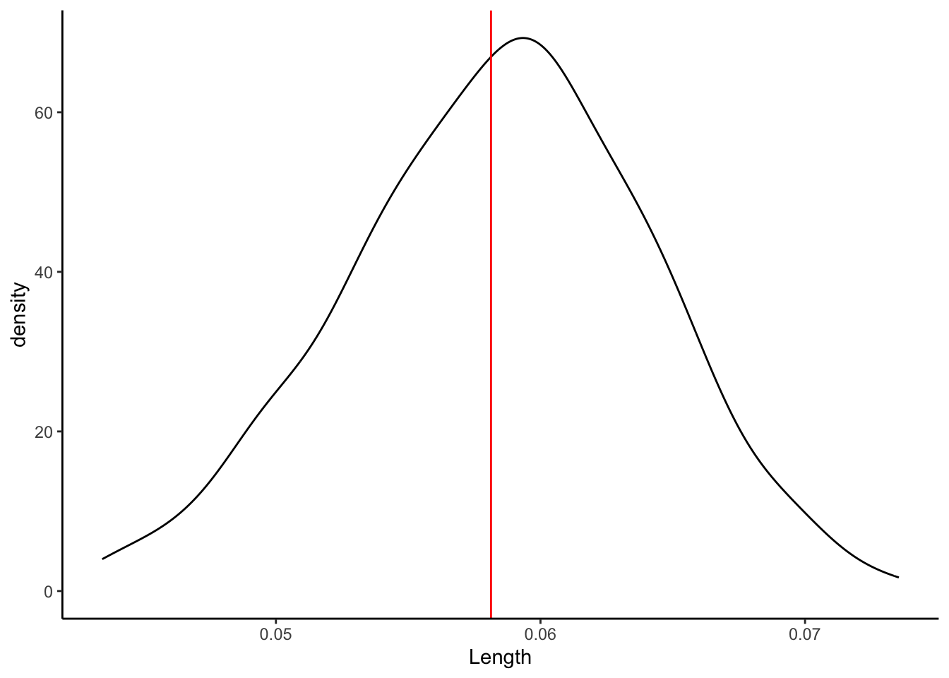
The sampling distribution is symmetric, unimodal, and shaped like a bell curve!
It is roughly centered at the slope calculated from our entire sample!
Most of the estimates lie within the range 0.04 to 0.075.
.
sample_models_boot %>%
summarize(sd(Length))# A tibble: 1 × 1
`sd(Length)`
<dbl>
1 0.00569Exercise 4: CLT distribution & standard error
Solution
coef(summary(fish_model)) Estimate Std. Error t value Pr(>|t|)
(Intercept) -1.13164542 0.213614796 -5.297598 3.617750e-07
Length 0.05812749 0.005227593 11.119359 6.641225e-22- Yes, the bootstrap distribution was roughly Normal / bell-shaped.
- Yes! They are basically identical! Both are about 0.005.
Exercise 5: Using the CLT
Solution
95%
100% - 95% = 5%
(100 - 99.7)/2 = 0.15% (Note that we divide by two here, because we only want those above 3 SEs, not either above or below!)
Exercise 6: CLT and the 68-95-99.7 Rule
Solution
68% of samples will produce \hat{\beta}_1 estimates within 1 st. err. of \beta_1
95% of samples will produce \hat{\beta}_1 estimates within 2 st. err. of \beta_1
99.7% of samples will produce \hat{\beta}_1 estimates within 3 st. err. of \beta_1
Exercise 7: Increasing sample size
Solution
Intuition, no wrong answer.
Exercise 8: 500 samples of size n
Solution
set.seed(155)
sample_models_50 <- map_df(1:500, function(i){
fish %>%
sample_n(size = 50, replace = TRUE) %>%
lm(Concen ~ Length, data = .) %>%
coef()
})
# Check it out
# Make sure that your first Intercept estimate is -1.9990216
head(sample_models_50)# A tibble: 6 × 2
`(Intercept)` Length
<dbl> <dbl>
1 -2.00 0.0795
2 -1.16 0.0589
3 -2.05 0.0811
4 -1.61 0.0697
5 -1.11 0.0542
6 -0.563 0.0423set.seed(155)
sample_models_20 <- map_df(1:500, function(i){
fish %>%
sample_n(size = 20, replace = TRUE) %>%
lm(Concen ~ Length, data = .) %>%
coef()
})
# Check it out
# Make sure that your first Intercept estimate is -2.2383596
head(sample_models_20)# A tibble: 6 × 2
`(Intercept)` Length
<dbl> <dbl>
1 -2.24 0.0847
2 -2.40 0.0884
3 -1.09 0.0559
4 -0.565 0.0431
5 -1.50 0.0696
6 -2.29 0.0894Exercise 9: Impact of sample size (part I)
Solution
The sample model lines become less and less variable from sample to sample.
# 500 sample models using samples of size 20
fish %>%
ggplot(aes(x = Length, y = Concen)) +
geom_smooth(method = "lm", se = FALSE) +
geom_abline(data = sample_models_20,
aes(intercept = `(Intercept)`, slope = Length),
color = "gray", size = 0.25) +
lims(x = c(25, 65), y = c(-1, 5))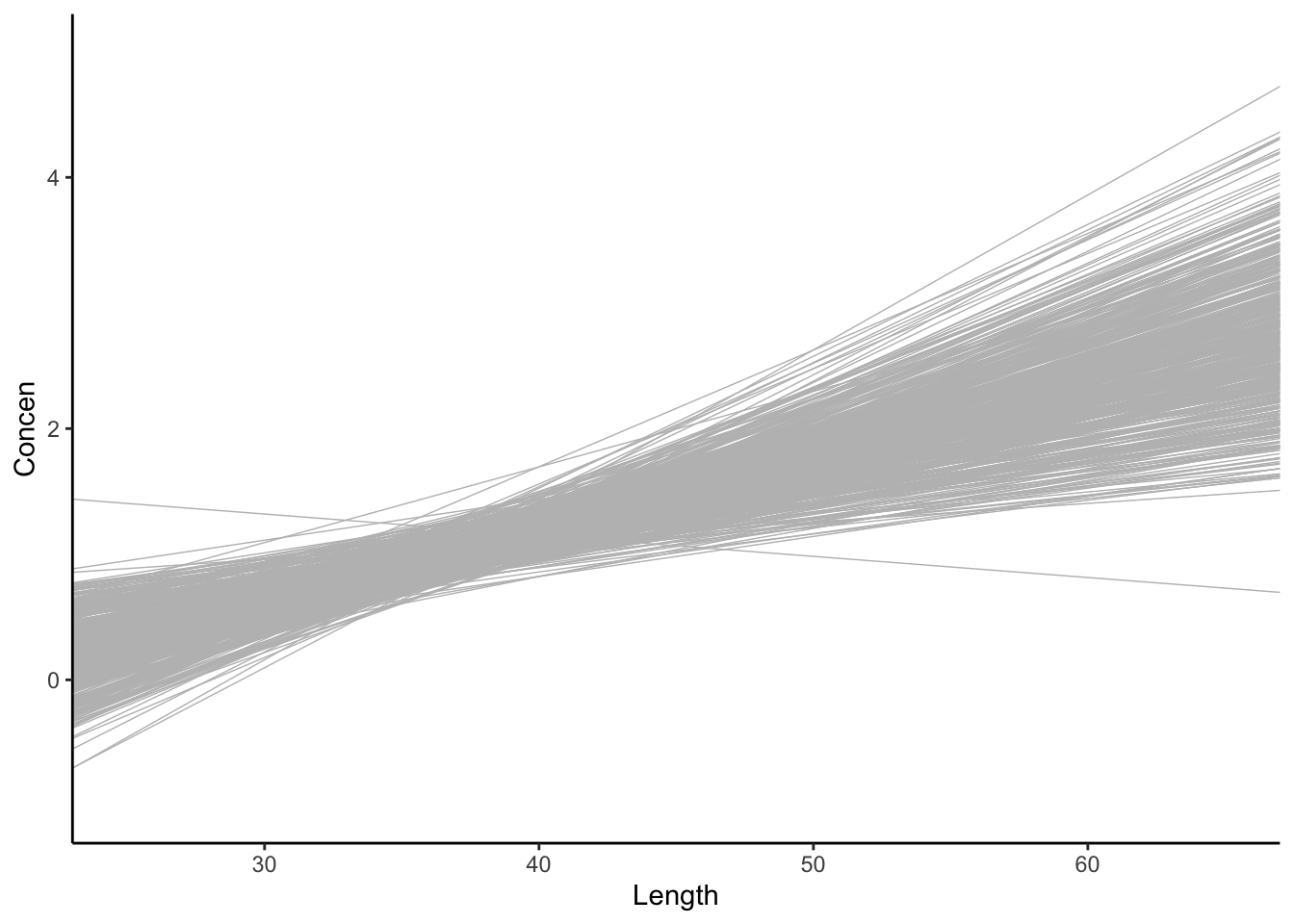
# 500 sample models using samples of size 50
fish %>%
  ggplot(aes(x = Length, y = Concen)) +
  geom_smooth(method = "lm", se = FALSE) +
  geom_abline(data = sample_models_50,
              aes(intercept = `(Intercept)`, slope = Length),
              color = "gray", size = 0.25) +
  lims(x = c(25, 65), y = c(-1, 5))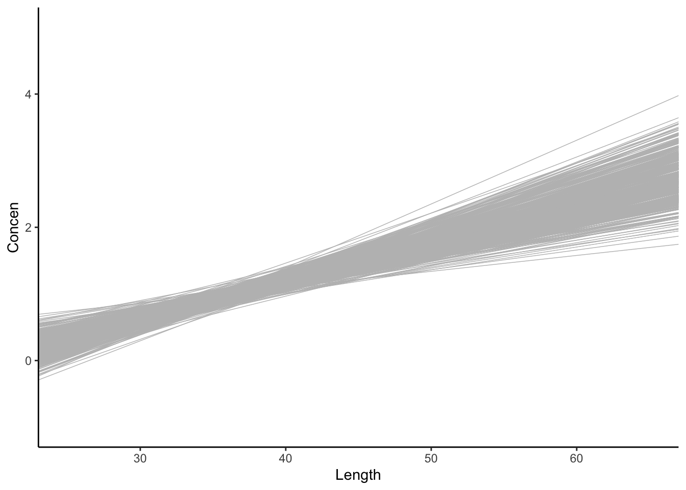
# 500 sample models using samples of size 171
fish %>%
  ggplot(aes(x = Length, y = Concen)) +
  geom_smooth(method = "lm", se = FALSE) +
  geom_abline(data = sample_models_boot,
              aes(intercept = `(Intercept)`, slope = Length),
              color = "gray", size = 0.25) +
  lims(x = c(25, 65), y = c(-1, 5))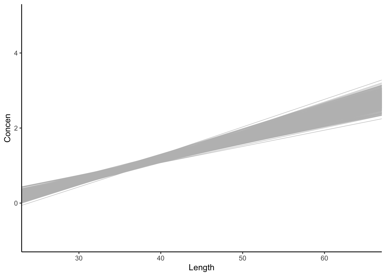
Exercise 10: Impact of sample size (part II)
Solution
No matter the sample size, the sample estimates are normally distributed around the same value (here the sample slope since we’re sampling from the sample). But as sample size increases, the variability of the sample estimates decreases.
# 500 sample slopes using samples of size 20
sample_models_20 %>%
  ggplot(aes(x = Length)) +
  geom_density() +
  lims(x = c(-0.01, 0.13), y = c(0, 70))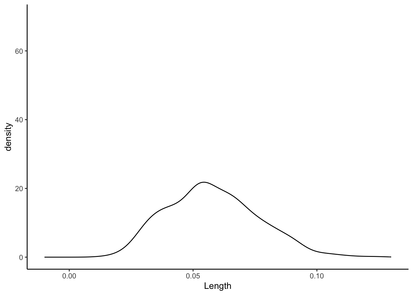
# 500 sample slopes using samples of size 50
sample_models_50 %>%
  ggplot(aes(x = Length)) +
  geom_density() +
  lims(x = c(-0.01, 0.13), y = c(0, 70))
# 500 sample slopes using samples of size 171
sample_models_boot %>%
  ggplot(aes(x = Length)) +
  geom_density() +
  lims(x = c(-0.01, 0.13), y = c(0, 70))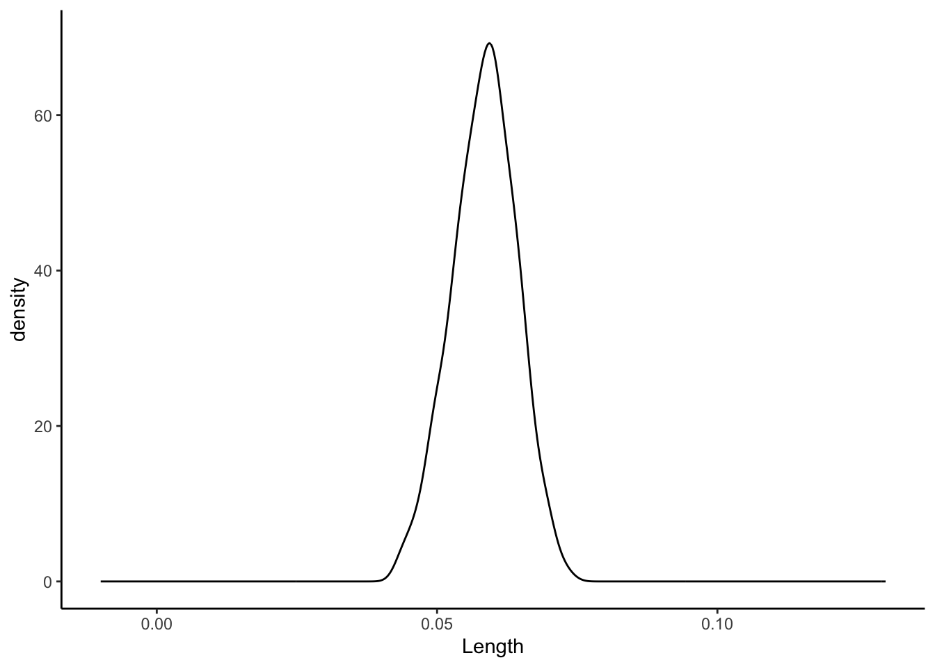
Exercise 11: Properties of sampling distributions
Solution
In light of your observations, complete the following statements about the sampling distribution of the sample slope.
For all sample sizes, the shape of the sampling distribution is roughly normal and the sampling distribution is roughly centered around 0.05813, the sample estimate from our original data.
As sample size increases:
The average sample slope estimate IS FAIRLY STABLE.
The standard error of the sample slopes DECREASES.Thus, as sample size increases, our sample slopes become MORE RELIABLE.