“Nested models” are models where the covariates of one model are a subset of another model. In other words, you can get to the smaller, nested model by setting some of the \beta’s to 0.
As an example, consider the following models for estimating the association between forced expiratory volume (FEV) and smoking status:
Here, even though Model 3 and Model 4 both contain smoke as explanatory variables, neither is nested in the other, since sex is not a part of Model 3, and height is not a part of Model 4.
F-test
NoteF-test test statistic
The F-test test statistic is not calculated like the t-test test statistic, thus cannot be interpreted the same way! Check out the theory box below to learn how this statistic is calculated.
NoteTheory Box: Calculating the F-test test statistic
Consider 2 models which we’ll estimate using n data points:
H_a: at least one of \beta_{k+1}, \beta_{k+2}, …, \beta_p is non-0
Then the F-test test statistic measures the additional residual error when using Model 2 vs Model 1, while accounting for the complexity of each model. The greater the test statistic, the greater the residuals when we simplify the model (go from Model 1 to Model 2), thus the more evidence we have to reject H_0:
Which of the following models are nested in the model E[A \mid B, C, D] = \beta_0 + \beta_1 D + \beta_2 B + \beta_3 C + \beta_4 B * C?
Model 1: E[A \mid B] = \beta_0 + \beta_1 B
Model 2: E[A \mid B, D] = \beta_0 + \beta_1 B + \beta_2 D
Model 3: E[B \mid C] = \beta_0 + \beta_1 C
Model 4: E[A \mid B, C, D] = \beta_0 + \beta_1 B + \beta_2 C + \beta_3 D
Model 5: E[A \mid B, C, D] = \beta_0 + \beta_1 C + \beta_2 B + \beta_3 D + \beta_4 B * D
Model 6: E[A \mid D] = \beta_0 + \beta_1 D
Consider the following models involving variables A, B, C, and D:
Model 1: E[A \mid B] = \beta_0 + \beta_1 B
Model 2: E[A \mid B, C] = \beta_0 + \beta_1 B + \beta_2 C
Model 3: E[A \mid B, C] = \beta_0 + \beta_1 B + \beta_2 C + \beta_3 BC
Model 4: E[A \mid C, D] = \beta_0 + \beta_1 C + \beta_2 D
Model 5: E[B \mid A] = \beta_0 + \beta_1 A
Model 6: E[B \mid A, C] = \beta_0 + \beta_1 A + \beta_2 C + \beta_3 AC
Determine for each of the following statements whether that statement is True or False.
Model 1 is nested in Model 2
Model 1 is nested in Model 3
Model 1 is nested in Model 4
Model 2 is nested in Model 3
Model 3 is nested in Model 2
Model 2 is nested in Model 6
What is one (numeric) way to compare the quality of nested models? Explain how you would determine which model is “better” based on this metric.
Example 2: t-tests & “overall” F-tests
To explore the relationship of casual bikeshare ridership with the day of week (weekend or weekday), feels like temperature (F), and actual temperature (F), let’s explore the following population model:
Call:
lm(formula = rides ~ weekend + temp_feel + temp_actual, data = bikes)

Residuals:
     Min       1Q   Median       3Q      Max
-1592.49  -252.52   -17.41   181.65  1973.12

Coefficients:
             Estimate Std. Error t value Pr(>|t|)
(Intercept) -1370.647     86.438 -15.857   <2e-16 ***
weekendTRUE   813.556     36.312  22.405   <2e-16 ***
temp_feel      11.997      8.712   1.377   0.1689
temp_actual    15.884      9.459   1.679   0.0935 .
---
Signif. codes:  0 '***' 0.001 '**' 0.01 '*' 0.05 '.' 0.1 ' ' 1

Residual standard error: 443.8 on 727 degrees of freedom
Multiple R-squared:  0.584, Adjusted R-squared:  0.5823
F-statistic: 340.2 on 3 and 727 DF,  p-value: < 2.2e-16
The “overall” F-test is reported in the bottom line of the summary(). What do you conclude from this test? NOTE: The F-test test statistic is not calculated in the same way as the t-test test statistic (it does not give the number of SE’s away from 0).
What do you conclude from the t-tests in the temp_feel and temp_actual rows of the summary() table?
Putting these together, what do you think? Which variables might be “good” predictors of ridership?
Example 3: F-tests for nested models
Let’s take the temperature variables out of the model:
# Refit bike_model_1 (just for ease of comparison)bike_model_1 <-lm(rides ~ weekend + temp_feel + temp_actual, bikes)# Fit a new modelbike_model_2 <-lm(rides ~ weekend, bikes)
Note that bike_model_2 is nested in bike_model_1. Thus we can compare them with the following F-test for nested models. State the hypotheses, p-value, and your conclusion.
# Put the smaller model first!!!anova(bike_model_2, bike_model_1)
Analysis of Variance Table

Model 1: rides ~ weekend
Model 2: rides ~ weekend + temp_feel + temp_actual
  Res.Df       RSS Df Sum of Sq      F    Pr(>F)
1    729 253858215
2    727 143177975  2 110680240 280.99 < 2.2e-16 ***
---
Signif. codes:  0 '***' 0.001 '**' 0.01 '*' 0.05 '.' 0.1 ' ' 1
A series of models and tests can provide more insight than one model or test alone! What did we learn about the relationship of rides with temp_feel and temp_actual from the above examples combined? Why do you think this happened? What would you do next?
Exercises
DIRECTIONS
Throughout this activity, test hypotheses at the 0.05 significance level.
Make all conclusions and interpretations in context.
CONTEXT
The MacGrades.csv dataset contains a sub-sample (to help preserve anonymity) of every grade assigned to a former Macalester graduating class. For each of the 6414 rows of data, the following information is provided (with a few missing values):
sessionID: A section ID number
sid: A student ID number
grade: The grade obtained, as a numerical value (i.e. an A is a 4, an A- is a 3.67, etc.)
dept: A department identifier (these have been made ambiguous to maintain anonymity)
level: The course level (e.g. 100-, 200-, 300-, and 600-)
sem: A semester identifier
enroll: The section enrollment
iid: An instructor identifier (these have been made ambiguous to maintain anonymity)
# Load packages & datalibrary(tidyverse)MacGrades <-read_csv("https://mac-stat.github.io/data/MacGrades.csv")%>%mutate(level =factor(level)) # make level a factor variablehead(MacGrades)
Exercise 1: Explore
NOTE: This exercise, since it’s exploratory in nature, can suck up a lot of time if you let them! For the sake of getting to the rest of the activity, please spend no more than ~5 minutes on this.
Hypothesize two relationships between the variables in the dataset (pick any two relationships you want!). Your response should be written in a paragraph form.
Response Put your response here
Explore the relationship between course grades and other variables in the data. Make two visualizations, and describe any patterns you observe.
Exercise 2: F-tests for grade vs level
Suppose we are interested in the relationship of student grade with the course level (categorical).
Using grade as your outcome variable, fit a linear regression model to investigate this question. Comment on the nature of the relationship between course level and student grades (this should not be a coefficient interpretation, but instead a description of a general trend, or lack thereof).
State the null and alternative hypotheses associated with the research question in part a.
H_0:
H_a:
What type of test do we need here: a t-test for a single model coefficient, the overall F-test, or a nested F-test?
What is the p-value associated with this hypothesis test? Do we have enough evidence to reject the null hypothesis, using a significance threshold of 0.05?
Exercise 3: F-tests for grade vs enrollment
Suppose we are interested in the relationship between course enrollment and student grades.
Again, use grade as your outcome variable, and fit a linear regression model to investigate this question.
State the null and alternative hypotheses associated with the research question in part a.
H_0:
H_a:
What type of test do we need here: a t-test for a single model coefficient, the overall F-test, or a nested F-test?
What is the p-value associated with this hypothesis test? Do we have enough evidence to reject the null hypothesis, using a significance threshold of 0.05?
Exercise 4: More F-tests
Suppose we are now interested in the association between course grade and enrollment for classes of the same level, i.e. when controlling for class level.
Write a model statement in the form E[Y | X] = ... that will produce a statistical model that will allow us to answer our scientific question. Replace Y and X, where appropriate, with response and predictor variables.
E[Y | X] = ___
Which coefficient(s) in your model is the one that is relevant to your research question?
What are the relevant null and alternative hypotheses that address the scientific question in part (a)?
Fit the model you wrote in part (a), calculate a p-value, and report the results of the hypothesis test in part (b).
Reflection
F-tests are useful when the null hypothesis you wish to test is such that more than one covariate is simultaneously equal to a specific number (typically zero). What scenarios, outside of those shown in this example, can you think of where a relevant scientific hypothesis you want to test involves more than one covariate being simultaneously equal to zero?
Extra Practice
Exercise 5: Repeat
Repeat Exercise 4, supposing we are instead interested in the association between course grade and course level for classes of the same enrollment.
Exercise 6: Guess the p-value
Consider 2 models of grades, 1 of which you’ve used before (but maybe named something else):
Using your notation from Exercise 4, state the hypotheses that would be tested by running anova(grades_model_B, grades_model_A). DO NOT YET RUN THIS CODE!
WITHOUT RUNNING THE anova() CODE: What will be the p-value reported by anova(grades_model_B, grades_model_A)? What’s your reasoning?
Check your intuition:
anova(grades_model_B, grades_model_A)
Exercise 7: But is it a “good” model?
In the above exercises, you should have concluded that, when controlling for the other, both course enrollments and course level are significantly associated with grades. But are they “good” predictors? Let’s explore grades_model_A in more depth.
The relationships of grade with enroll and level are statistically significant, but are they practically significant / contextually meaningful?
Grades vary from student to student within and across courses. What percentage of this variation is explained by course enrollments and level?
Putting this all together, what’s your overall conclusion about the relationship here?
Exercise 8: Reference categories
Our final research question pertains to whether or not there is a relationship between course grade and department. Again, use course grade as the outcome variable in your linear regression model.
State the null and alternative hypotheses in colloquial language associated with the relevant hypothesis test.
H_0:
H_a:$
Fit a linear regression model, and conduct your hypothesis testing procedure to answer the research question posed in this Exercise. State your conclusions accordingly (you do not need to interpret any regression coefficients, just state and interpret the results of your hypothesis test!).
Are any of the individual department p-values significant? What do these p-values tell us, and why is this not contradictory to your answer in part (b)?
Wrap Up
Finish and study the activity!
Project Milestone 2 due Friday night
PS 8 due next Monday
Reminders:
Remember the important basics: complete activities, ask for help, study on a regular basis, start assignments early.
If you miss class on a project day, it’s your responsibility to communicate with your group, find out what you missed, and make equivalent contributions outside of class. If missing class on project days becomes a pattern, it will impact your project grade.
Your final project grade will reflect your individual engagement and contributions to the project. You are not expected to be perfect. Rather, you should put effort, attention, and reflection into the following areas:
communication
contributing to group discussions
including all other group members in discussion
creating a space where others felt comfortable sharing ideas and mistakes
communicating with your group outside class
report contributions
contributing to the content / analysis in the report
contributing to the writing of the report
contributing to the editing of the report
Solutions
Warm Up
Example 1: Nested Models
Solution
Models 1, 2, 4 and 6.
Model 1 is nested in Model 2 TRUE
Model 1 is nested in Model 3 TRUE
Model 1 is nested in Model 4 FALSE
Model 2 is nested in Model 3 TRUE
Model 3 is nested in Model 2 FALSE
Model 2 is nested in Model 6 FALSE
You could compare the Adjusted R^2 values from each model, and note that the one with a higher adjusted R^2 is better by this metric. Multiple R^2 would not be a good metric, because the larger model (within the nesting structure) will always have a higher R^2 value.
Call:
lm(formula = rides ~ weekend + temp_feel + temp_actual, data = bikes)

Residuals:
     Min       1Q   Median       3Q      Max
-1592.49  -252.52   -17.41   181.65  1973.12

Coefficients:
             Estimate Std. Error t value Pr(>|t|)
(Intercept) -1370.647     86.438 -15.857   <2e-16 ***
weekendTRUE   813.556     36.312  22.405   <2e-16 ***
temp_feel      11.997      8.712   1.377   0.1689
temp_actual    15.884      9.459   1.679   0.0935 .
---
Signif. codes:  0 '***' 0.001 '**' 0.01 '*' 0.05 '.' 0.1 ' ' 1

Residual standard error: 443.8 on 727 degrees of freedom
Multiple R-squared:  0.584, Adjusted R-squared:  0.5823
F-statistic: 340.2 on 3 and 727 DF,  p-value: < 2.2e-16
H_0: \beta_1 = \beta_2 = \beta_3 = 0 H_a: at least 1 of \beta_1, \beta_2, \beta_3 is not 0
We rejectH_0 (p-value < 0.05). We have statistically significant evidence that at least 1 of weekend, temp_feel, or temp_actual are associated with rides.
.
H_0: \beta_2 = 0 H_a: \beta_2 \ne 0
We fail to rejectH_0 (p-value > 0.05). We do not have statistically significant evidence that when controlling for weekend and temp_actual, there’s an association between rides and temp_feel. That is, if we already know weekend and temp_actual, then temp_feel doesn’t provide significantly more information about rides.
Similarly, we do not have statistically significant evidence that when controlling for weekend and temp_feel, there’s an association between rides and temp_actual.
It might seem like temperature variables aren’t good predictors of ridership, but weekend status is. As we’ll learn, that’s not correct!!
Example 3: F-tests for nested models
Solution
Let’s take the temperature variables out of the model:
# Refit bike_model_1 (just for ease of comparison)bike_model_1 <-lm(rides ~ weekend + temp_feel + temp_actual, bikes)# Fit a new modelbike_model_2 <-lm(rides ~ weekend, bikes)
H_0: \beta_2 = \beta_3 = 0 H_a: at least 1 of \beta_2 and \beta_3 are non-0
We rejectH_0 (p-value < 0.05). We have statistically significant evidence that when controlling for weekend status, rides is associated with at least one of temp_feel or temp_actual. That is, even if we already know weekend status, at least one of temp_actual or temp_feel provides significantly new information about rides.
temp_feel and temp_actual aren’t significant when the other is in the model, but at least 1 of these is significantly associated with rides. These predictors are likely multicollinear – thus if we already have one of them in our model, we likely don’t need the other. Our next step would be to take 1 out of the model and see what happens to the significance of the other.
Exercises
Exercise 1: Explore
Solution
Answers will vary a lot from student to student!
It is reasonable to assume that course grade varies by department as well as course level and instructor. Certain instructors may grade more strictly (or curve more) than others, and similarly, this can vary across department due to cultural norms within the department. As the level of a course gets higher, I would expect grades to perhaps get lower, since courses with higher numbers are expected to be more difficult. Then again, students perhaps “care” more about such courses, and may put in more effort to get a higher grade. I doubt semester plays a significant role in determining course grades, though it is possible that Fall semester first-years or Spring semester seniors have worse grades, on average. We don’t have course year as a variable in our data, so we would be unable to examine this relationship. As enrollment in a course goes up, I would expect grades to decrease, since professors have less time to dedicate to individual students when course enrollment is high.
Explore the relationship between course grades and other variables in the data. Make at least four visualizations, and describe any patterns you observe.
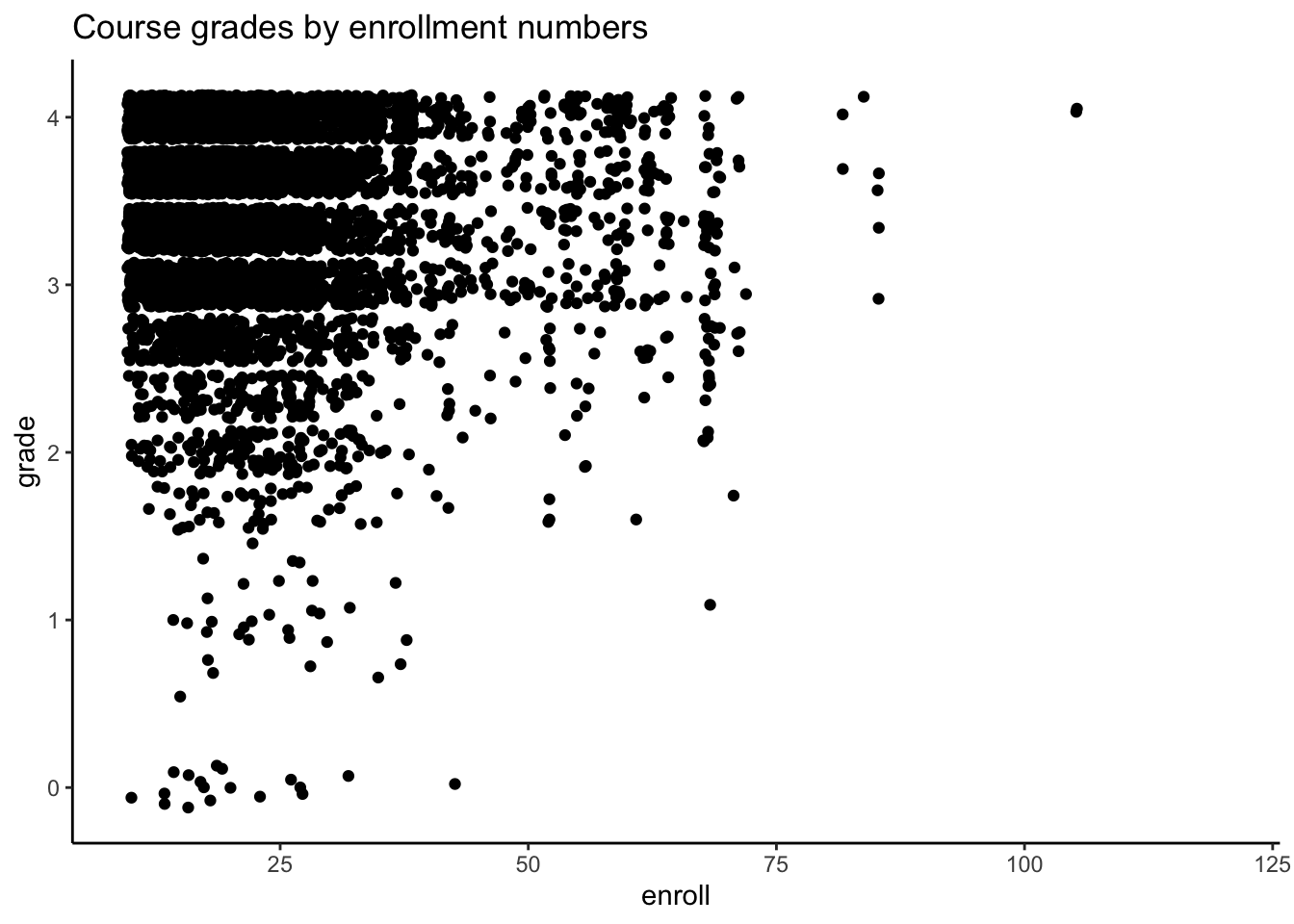
# Exploratory plots# course grade vs. enrollmentMacGrades %>%ggplot(aes(enroll, grade)) +geom_jitter() +theme_classic() +ggtitle("Course grades by enrollment numbers")
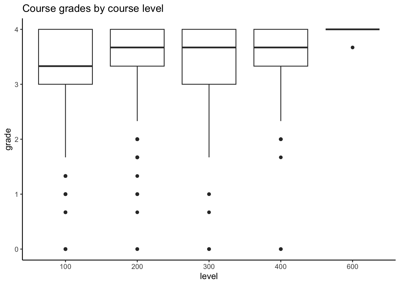
# course grade vs. levelMacGrades %>%mutate(level =factor(level)) %>%ggplot(aes(y = grade, x = level)) +geom_boxplot() +ggtitle("Course grades by course level")
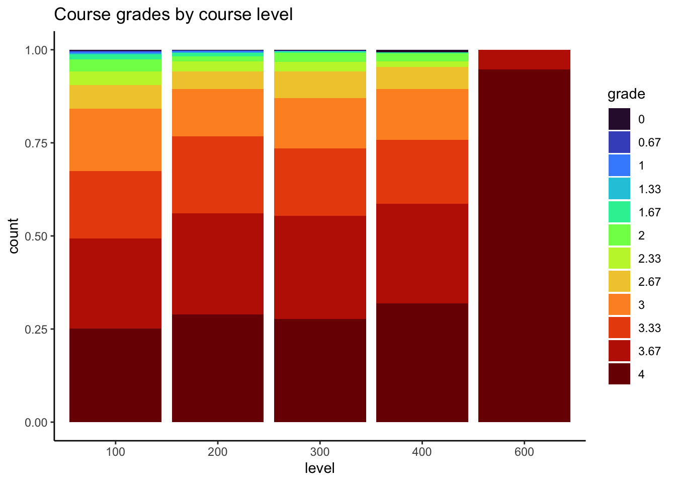
# course grade vs. level (treating grade as categorical)MacGrades %>%filter(!is.na(grade)) %>%mutate(level =factor(level),grade =factor(grade)) %>%ggplot(aes(x = level, fill = grade)) +geom_bar(position ="fill") +scale_fill_viridis_d(option ="H") +theme_classic() +ggtitle("Course grades by course level")
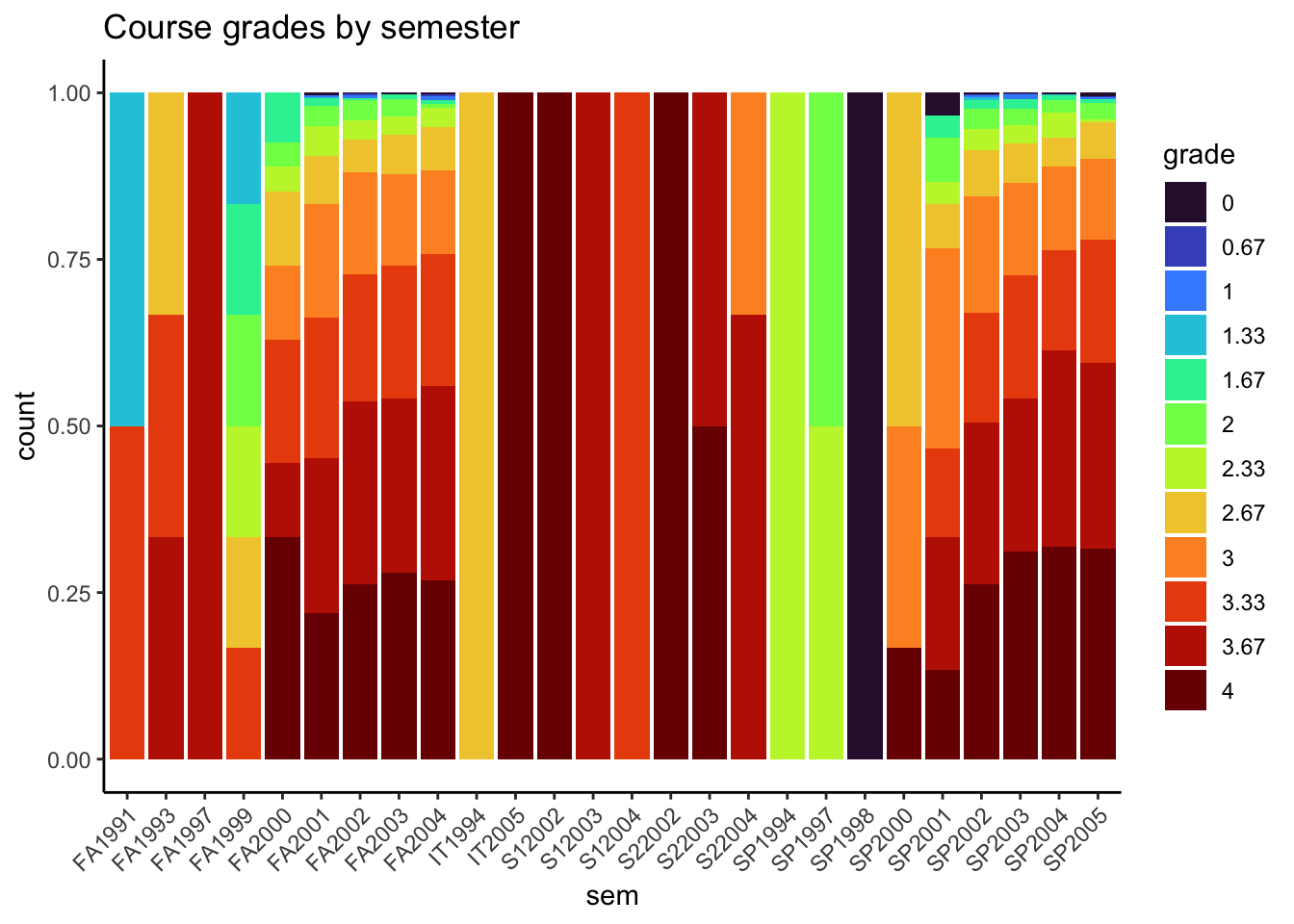
# course grade vs. semesterMacGrades %>%filter(!is.na(grade)) %>%mutate(grade =factor(grade)) %>%ggplot(aes(x = sem, fill = grade)) +geom_bar(position ="fill") +scale_fill_viridis_d(option ="H") +theme_classic() +ggtitle("Course grades by semester") +theme(axis.text.x =element_text(angle =45, hjust =1))
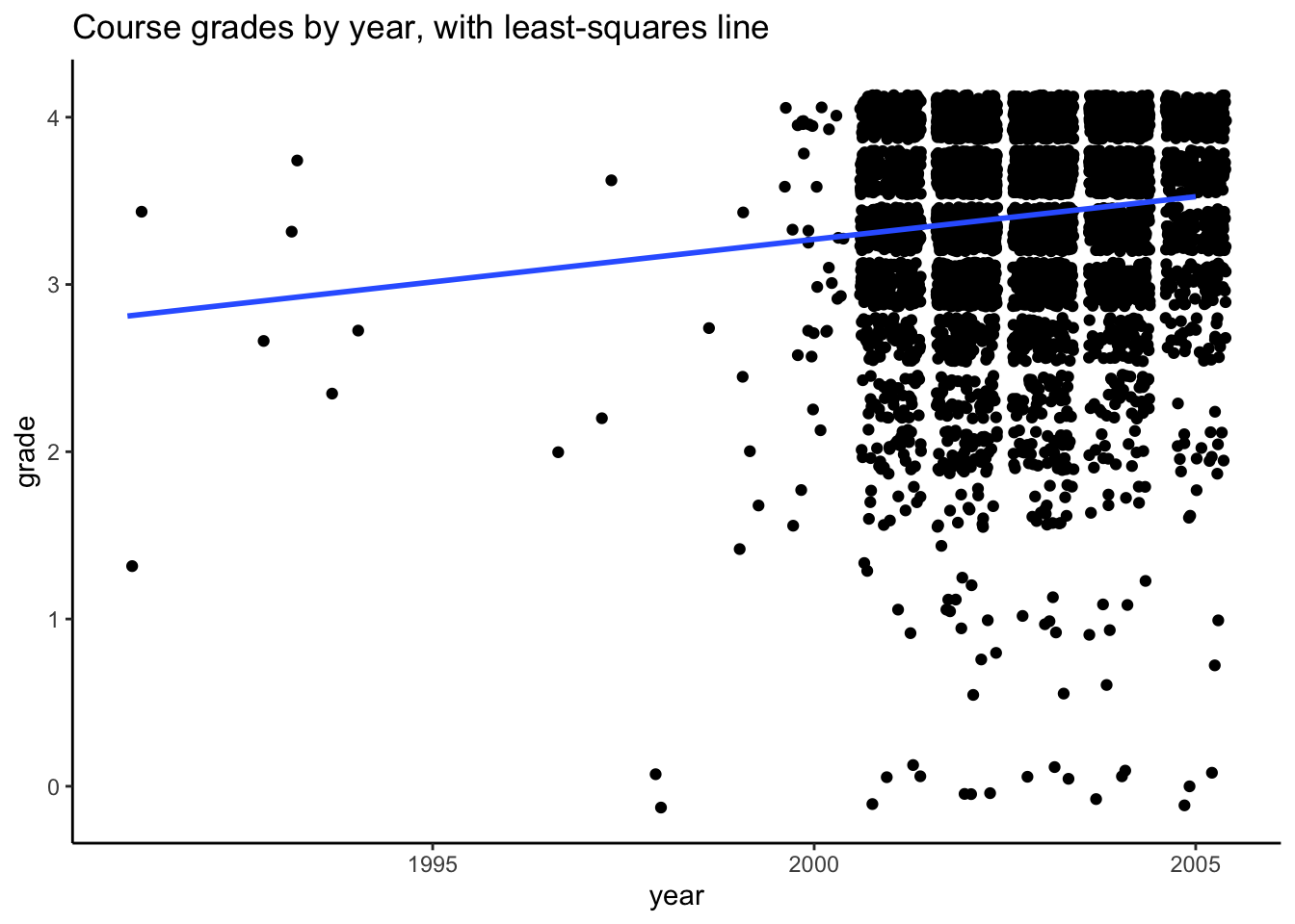
# Let's do something fancy and check out how grades have changed over time... this will require# some string manipulationMacGrades$year <- MacGrades$sem %>%str_replace("FA", "") %>%str_replace("SP", "") %>%str_replace("S1", "") %>%str_replace("S2", "") %>%str_replace("IT", "") %>%as.numeric()MacGrades %>%ggplot(aes(year, grade)) +geom_jitter() +geom_smooth(method ="lm", se =FALSE) +theme_classic() +ggtitle("Course grades by year, with least-squares line")
In general, course grades seem to be associated with enrollment numbers. Specifically, when enrollments are greater than 50, we see very few students receiving a course grade lower than a 2.0, which is different than when enrollments are fewer than 50 students. There does not appear to be a clear relationship between course grade and course level, with the exception of 600-level courses. In these cases, every student received either an A or A-. It does seem like the proportion of students who received lower than a 2.67 is greater for 100-level courses than the other course levels.
Exercise 2: F-tests for grade vs level
Solution
mod <-lm(grade ~ level, data = MacGrades)summary(mod)
Call:
lm(formula = grade ~ level, data = MacGrades)

Residuals:
    Min      1Q  Median      3Q     Max
-3.5108 -0.3620  0.2088  0.4892  0.6380

Coefficients:
             Estimate Std. Error t value Pr(>|t|)
(Intercept) 3.3123669  0.0173797 190.588  < 2e-16 ***
level       0.0004962  0.0000776   6.394 1.75e-10 ***
---
Signif. codes:  0 '***' 0.001 '**' 0.01 '*' 0.05 '.' 0.1 ' ' 1

Residual standard error: 0.5925 on 5707 degrees of freedom
  (437 observations deleted due to missingness)
Multiple R-squared:  0.007112,  Adjusted R-squared:  0.006938
F-statistic: 40.88 on 1 and 5707 DF,  p-value: 1.746e-10
We observe that as course level goes up, course grades also tend to increase on average.
.
H_0: \beta_1 = \beta_2 = \beta_3 = \beta_4 = 0
H_1: \text{At least one of } \beta_1, \beta_2, \beta_3, \beta_4 \neq 0
In words, the null is that there is no relationship between course level and course grades, and the alternative is that there is some relationship (either positive or negative) between course level and course grades.
overall F-test
The p-value associated with this hypothesis test is 9.713 x 10^{-13}. We do have enough evidence to reject the null hypothesis. The difference in grades by level is not statistically significant.
Exercise 3: F-tests for grade vs enrollment
Solution
mod <-lm(grade ~ enroll, data = MacGrades)summary(mod)
Call:
lm(formula = grade ~ enroll, data = MacGrades)

Residuals:
    Min      1Q  Median      3Q     Max
-3.4529 -0.3871  0.2265  0.5534  0.8448

Coefficients:
              Estimate Std. Error t value Pr(>|t|)
(Intercept)  3.4842350  0.0173790 200.485  < 2e-16 ***
enroll      -0.0031336  0.0006683  -4.689 2.81e-06 ***
---
Signif. codes:  0 '***' 0.001 '**' 0.01 '*' 0.05 '.' 0.1 ' ' 1

Residual standard error: 0.5934 on 5707 degrees of freedom
  (437 observations deleted due to missingness)
Multiple R-squared:  0.003838,  Adjusted R-squared:  0.003664
F-statistic: 21.99 on 1 and 5707 DF,  p-value: 2.806e-06
H_0: \beta_1 = 0
H_1: \beta_1 \neq 0
t-test (an overall F-test would also work since there’s only one non-intercept coefficient in this model!!!)
The p-value associated with this hypothesis test is 2.806 x 10^{-06}. We do have enough evidence to reject the null hypothesis. Note that this p-value could be obtained from either the overall model fit or from the individual coefficient for enroll (they are the same). They may be ever so slightly different when there are few observations in your dataset, but when there are a lot, they will be exactly identical.
The relevant coefficient that answers our scientific question is \beta_1, or the coefficient that corresponds to enrollment.
The relevant null and alternative hypotheses are:
H_0: \beta_1 = 0
H_1: \beta_1 \neq 0
We do not need to conduct an F-test to complete this hypothesis testing procedure, since our hypothesis involves only a single regression coefficient.
mod <-lm(grade ~ enroll + level, data = MacGrades)summary(mod)
Call:
lm(formula = grade ~ enroll + level, data = MacGrades)

Residuals:
    Min      1Q  Median      3Q     Max
-3.5201 -0.3602  0.1930  0.5165  0.7600

Coefficients:
              Estimate Std. Error t value Pr(>|t|)
(Intercept)  3.376e+00  2.656e-02 127.088  < 2e-16 ***
enroll      -2.185e-03  6.896e-04  -3.168  0.00154 **
level        4.311e-04  8.021e-05   5.375 7.98e-08 ***
---
Signif. codes:  0 '***' 0.001 '**' 0.01 '*' 0.05 '.' 0.1 ' ' 1

Residual standard error: 0.592 on 5706 degrees of freedom
  (437 observations deleted due to missingness)
Multiple R-squared:  0.008856,  Adjusted R-squared:  0.008508
F-statistic: 25.49 on 2 and 5706 DF,  p-value: 9.512e-12
We have statistically significant evidence of a relationship between enrollment and course grade, for courses of the same level (p = 0.001058). We reject the null hypothesis that there is no relationship between enrollment and course grade, adjusting for course level.
Exercise 5: Repeat
Solution
Our model statement is identical to that in Exercise 4, but the relevant coefficients are \beta_2, \beta_3, \beta_4, and \beta_5.
The relevant null and alternative hypotheses are:
H_0: \beta_2 = \beta_3 = \beta_4 = \beta_5 = 0
H_1: \text{At least one of } \beta_2, \beta_3, \beta_4, \beta_5 \neq 0
We do need to conduct an F-test to complete this hypothesis testing procedure, since our hypothesis involves more than one regression coefficient.
# Same model as in Question 10, we just now need to do an F-test!mod <-lm(grade ~ enroll + level, data = MacGrades)smaller_mod <-lm(grade ~ enroll, data = MacGrades)anova(smaller_mod, mod)
Analysis of Variance Table

Model 1: grade ~ enroll
Model 2: grade ~ enroll + level
  Res.Df    RSS Df Sum of Sq      F    Pr(>F)
1   5707 2009.8
2   5706 1999.7  1    10.123 28.887 7.977e-08 ***
---
Signif. codes:  0 '***' 0.001 '**' 0.01 '*' 0.05 '.' 0.1 ' ' 1
We have statistically significant evidence of a relationship between course level and course grade, for courses of the same enrollment (p = 2.19 \times 10^{-10}). We reject the null hypothesis that there is no relationship between course level and course grade, adjusting for enrollment.
Call:
lm(formula = grade ~ level, data = MacGrades)

Residuals:
    Min      1Q  Median      3Q     Max
-3.5108 -0.3620  0.2088  0.4892  0.6380

Coefficients:
             Estimate Std. Error t value Pr(>|t|)
(Intercept) 3.3123669  0.0173797 190.588  < 2e-16 ***
level       0.0004962  0.0000776   6.394 1.75e-10 ***
---
Signif. codes:  0 '***' 0.001 '**' 0.01 '*' 0.05 '.' 0.1 ' ' 1

Residual standard error: 0.5925 on 5707 degrees of freedom
  (437 observations deleted due to missingness)
Multiple R-squared:  0.007112,  Adjusted R-squared:  0.006938
F-statistic: 40.88 on 1 and 5707 DF,  p-value: 1.746e-10
H_0:\beta_1 = 0 H_a:\beta_1 \ne 0
will vary
The p-value is 0.001058, which is the same as the t-test on the enroll coefficient in summary(grades_model_A). The p-value is the same because they’re testing the same hypotheses!
anova(grades_model_B, grades_model_A)
Analysis of Variance Table

Model 1: grade ~ level
Model 2: grade ~ enroll + level
  Res.Df    RSS Df Sum of Sq      F   Pr(>F)
1   5707 2003.2
2   5706 1999.7  1    3.5176 10.037 0.001542 **
---
Signif. codes:  0 '***' 0.001 '**' 0.01 '*' 0.05 '.' 0.1 ' ' 1
Exercise 7: But is it a “good” model?
Solution
The enroll predictor doesn’t seem practically meaningful (to me!). There’s a small decrease in average grade per enrollment (0.002) when controlling for level. Given the small class sizes at Mac, this per-enrollment decrease wouldn’t “add up” to a meaningful drop in average grade in most courses.
But the level predictor does seem practically meaningful (to me!). For example, an increase of 0.6 in the average grade from a 100-level to a 600-level course, when controlling for enrollment, is a big jump on the GPA scale.
Only 1.271%. (This is the R-squared value.)
It seems that course grades are associated with course level and enrollments, but these factors are not “good” predictors of grades.
Exercise 8: Reference categories
Solution
H0: There is no relationship between course grade and department.
H1: There is some relationship between course grade and department.
mod <-lm(grade ~ dept, data = MacGrades)summary(mod)
We have statistically significant evidence of a relationship between department and course grades at a significance level of 0.05 (p-value < 2.2 x 10^{-16}). We reject the null hypothesis that there is no relationship between course grade and department.
None of the individual p-values for department are significant! These p-values tell us about whether or not there is a statistically significant difference in course grades between each respective department and the reference department (Department “A”). This doesn’t contradict our answer to part (b) because there are different hypothesis tests that answer different questions!