22 More confidence intervals

Settling In

Hand in Quiz 2 revisions.
Open up the course site:
- Type up your notes in “22-confidence-intervals-2-notes.qmd”.
Sit with people that ARE in your project group.
- Take the first 10 minutes of class to share what you found for Milestone 1. See if you can coalesce around one research question.

Fall 2026 registration (starting April 20th)
- “Shiny App for Fall Courses”
- COMP/STAT 112: Intro to Data Science Focuses on data storytelling (not modeling) and the necessary RStudio tools (more of the focus than in STAT 155).
- STAT 253: Statistical Machine Learning
  - The sequel to this course. Expands upon the foundational tools needed to make meaning from data:
    - types of tasks: regression (Y is quantitative), classification (Y is categorical), and unsupervised learning (no Y!)
    - types of tools for those tasks: parametric vs nonparametric tools (when models like linear regression are too rigid)
    - model selection (determining which variables to include, and how to include them)
    - model evaluation (bias-variance trade-off, cross validation)
  - This is a survey course: roughly 1 new algorithm / big concept per class, emphasizing breadth over depth.
  - Algorithms: linear regression, logistic regression, LASSO, KNN, trees, forests, bagging, hierarchical clustering, K-means clustering, principal components analysis (PCA), and more

Recap

Statistical superpowers

When using our sample data to make estimates about the population, we can do better than providing a single best guess. We can obtain a range of guesses that better captures our understanding and reflects the potential error in our estimate. This is a confidence interval.

Learning goals

By the end of this lesson, you should be able to:

Construct (approximate) confidence intervals by hand using the 68-95-99.7 rule
Construct exact confidence intervals in R
Interpret confidence intervals in context by referring to the coefficient of interest
Use confidence intervals to make statements about whether there appear to be true population relationships, changes, and differences

Additional resources

Required:

Video : Introduction to Confidence Intervals
Reading: Section 7 Introduction, Section 7.1, Section 7.2 (stop when you get to 7.2.4.3 Confidence Intervals for Prediction) in the STAT 155 Notes

Optional:

Video 2: Confidence Intervals: Construction and Interpretation

Confidence Intervals

Confidence interval for \beta

To communicate and contextualize the potential error in \hat{\beta}, we can calculate a confidence interval (CI) for \beta. This CI:

reflects the potential error in \hat{\beta}
provides a range of plausible values for \beta, i.e. an interval estimate
allows us to draw fair conclusions about the population using data from our sample!

Using the CLT, an approximate 95% confidence interval for \beta can be calculated by the formula below. (More precise calculations are provided in RStudio.)

\hat{\beta} \pm 2 \text{SE}(\hat{\beta})

Interpreting a CI

Let (a, b) represent the 95% CI for \beta.

Correct: We are 95% confident that \beta is between a and b.
Incorrect: There’s a 95% chance that \beta falls between a and b.
- Nope! \beta is either in there, or it isn’t. No probability involved.
- It is either in the interval or not, so the probability is 1 or 0.
Incorrect: There’s a 95% chance that sample estimate \hat{\beta} is between a and b.
- Nope! We have no uncertainty about \hat{\beta} – we know exactly what it is and it’s always in the interval by construction.

What does “95% confidence” mean?!

Important nuances:
- \beta is “fixed”, i.e. not random. There’s a fixed, “true” value of \beta, we just don’t know what it is. Thus we can’t make probability statements about \beta.
- \hat{\beta} is random (it varies from sample to sample, depending upon what sample we happen to get). Thus we can make probability statements about \hat{\beta}.
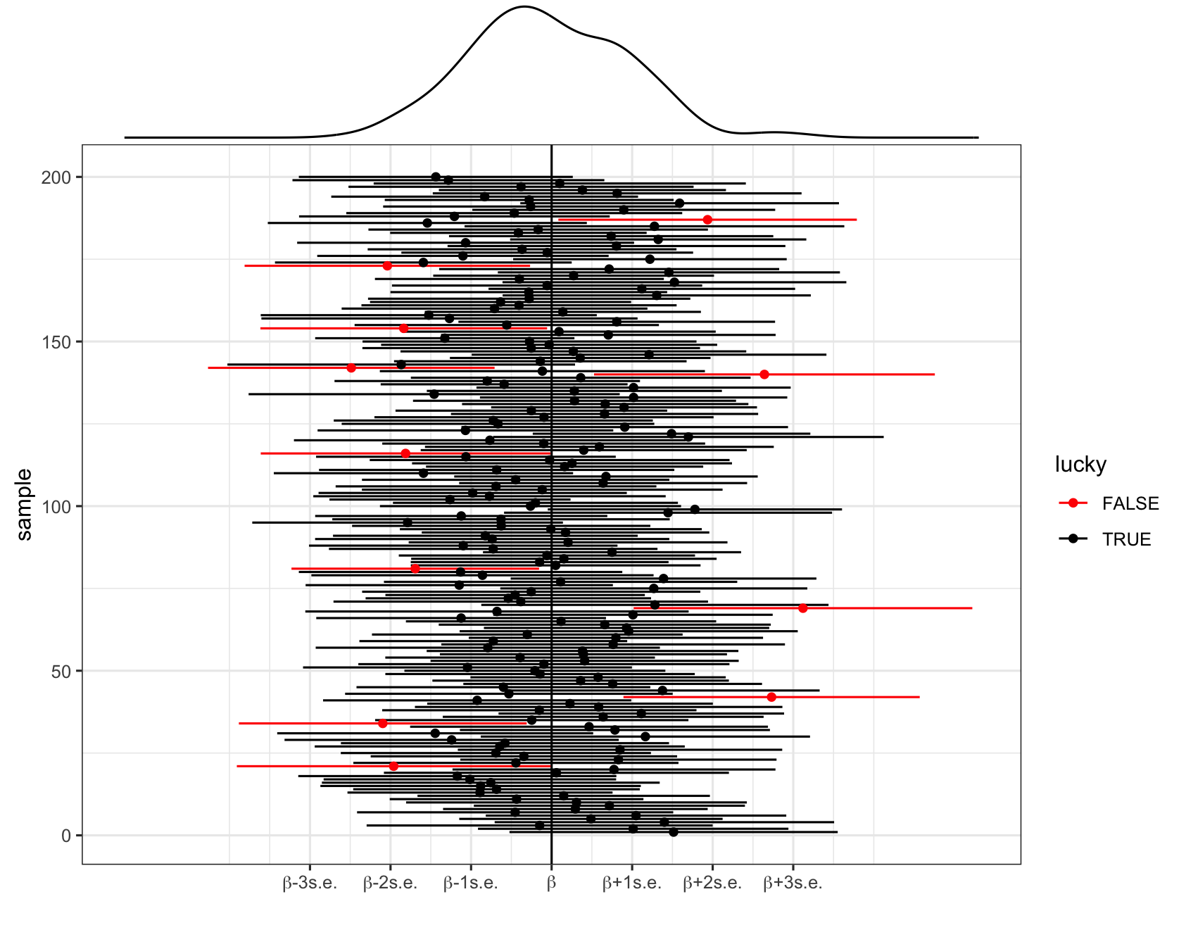
Thus “95% confidence” references the randomness and variability in \hat{\beta} and the interval construction process, not \beta: 95% of all possible samples will produce 95% CIs that contain the true \beta value.
In pictures: 200 different 95% CIs for \beta calculated from 200 different samples. Each sample produces a different estimate \hat{\beta} (dot) hence a different 95% CI for \beta (horizontal line). Roughly 95% of these contain \beta (the black intervals) and roughly 5% do not (the red intervals).

Exercises

Exercise 1: Confidence Interval Review

In the first set of exercises, we’ll model the time it takes to complete a mountain hike. To begin, let’s explore the relationship of completion time (in hours) by hike length (in miles):

E[time | length] = \beta_0 + \beta_1 length

A sample estimate of this population model, obtained using our data on hiking trails in the Adirondack mountains, is below:

E[time | length] = \hat{\beta}_0 + \hat{\beta}_1 length = 2.048 + 0.684 length

# Import the data & load important packages
library(tidyverse)
peaks <- read.csv("https://mac-stat.github.io/data/high_peaks.csv")

# Model the relationship
peaks_model_1 <- lm(time ~ length, data = peaks)
coef(summary(peaks_model_1))

# Visualize the relationship
peaks %>% 
  ggplot(aes(y = time, x = length)) + 
  geom_point() + 
  geom_smooth(method = "lm")

Part a

\hat{\beta}_1 simply provides a point estimate, or our single best guess, of \beta_1. To also produce an interval estimate, use the 68-95-99.7 Rule to approximate a 95% CI for \beta_1.

Part b

We can calculate a more accurate CI by applying the confint() function to our model. Your approximation from Part a should be close!

confint(peaks_model_1, level = 0.95)

Exercise 2: Interpreting the CI

Part a

Interpreting the CI for \beta_1 in context requires that we can interpret \beta_1 itself! So how can we interpret \beta_1 (in general, without assuming a specific value for the unknown \beta_1)? Choose 1.

\beta_1 measures the expected completion time for hikes that are 0 miles long
\beta_1 measures the difference in the expected completion time for hikes that long vs hikes that aren’t long
\beta_1 measures the change in the expected completion time for each additional 1 mile in length

Part b

Per the previous exercise: “We are 95% confident that \beta_1 is between 0.56 and 0.81”. Interpret this CI in context, drawing on your answer to Part a.

Exercise 3: time versus elevation

Next, let’s explore the relationship between the completion time and maximum elevation of a hike (in feet):

E[time | elevation] = \beta_0 + \beta_1 elevation

We can gain insight into this relationship using our sample data:

# Model the relationship
peaks_model_2 <- lm(time ~ elevation, data = peaks)

# Get confidence intervals
confint(peaks_model_2, level = 0.95)

# Plot the sample model
ggplot(peaks, aes(y = time, x = elevation)) + 
  geom_point() + 
  geom_smooth(method = "lm")

What can we conclude from both the CI for \beta_1 and the confidence bands in the plot above?

Exercise 4: time versus rating

Next, let’s explore the relationship between the completion time and hike rating (difficult, easy, or moderate):

E[time | rating] = \beta_0 + \beta_1 ratingeasy + \beta_2 ratingmoderate

PAUSE: Before analyzing this model, pause to reflect on what \beta_0, \beta_1, and \beta_2 mean in this context. We can gain insight into these coefficients using our sample data:

# Visualize the relationship
ggplot(peaks, aes(y = time, x = rating)) + 
  geom_boxplot()

# Model the relationship
peaks_model_3 <- lm(time ~ rating, data = peaks)

# Obtain CIs for the model coefficients
confint(peaks_model_3)

Part a

How can we interpret the confidence interval for \beta_2, the ratingmoderate coefficient: (-5.92, -3.19)? We’re 95% confident that… (Choose 1)

the average completion time of a moderate hike is between 3.19 and 5.92 hours
the average completion time of a moderate hike is between 3.19 and 5.92 hours less than that of a difficult hike
the average completion time of moderate hikes in our sample was between 3.19 and 5.92 hours less than that of difficult hikes in our sample

Part b

How can we interpret the confidence interval for the intercept \beta_0: (13.8, 16.2)? We’re 95% confident that… (Choose 1)

the average completion time of a hike with a 0 rating is between 13.8 and 16.2 hours.
the average completion time of a difficult hike is between 13.8 and 16.2 hours.
the average completion time of a hike is between 13.8 and 16.2 hours.
the average completion time of a difficult hike is between 13.8 and 16.2 hours more than that of an easy hike.

Exercise 5: Multiple logistic regression REVIEW

Let’s turn our attention to weather in 3 Australia locations, Hobart, Uluru, and Wollongong: When controlling for location, is today’s 9am humidity level (0-100%) a “significant” predictor of whether or not it will rain tomorrow? The following population model represents this relationship:

log(odds of rain_tmrw) = \beta_0 + \beta_1 locationUluru + \beta_2 locationWollongong + \beta_3 humidity9am

Below we build a sample model using a sample of 500 data points:

# NOTE: We'll take a sub-sample of 500 days for TEACHING PURPOSES ONLY
# In practice, we'd use all data in our sample :)
set.seed(155)
weather <- read_csv("https://mac-stat.github.io/data/weather_3_locations.csv") %>% 
  mutate(rain_tmrw = (raintomorrow == "Yes")) %>% 
  sample_n(size = 500, replace = FALSE)

# Build the sample model
weather_model_1 <- glm(rain_tmrw ~ location + humidity9am, data = weather, family = "binomial")
coef(summary(weather_model_1))

# Exponentiate the coefficients
exp(coef(weather_model_1))

Part a

Why are we using logistic regression?

Part b

Interpret \hat{\beta}_0, the estimated intercept, on the odds scale. Circle any option that’s correct! On a day with 0 humidity at 9am in Hobart…

The odds of rain are 0.015.
The chance of rain is 0.015.
The chance of rain is 1.5% as high as the chance of no rain.
The odds of rain increase by 0.15%.

Part c

Interpret \hat{\beta}_1, the estimated locationUluru coefficient, on the odds scale. When controlling for 9am humidity levels…

the odds of rain are 0.60 in Uluru.
the odds of rain are 60% higher in Uluru than in Hobart.
the odds of rain in Uluru are 60% as high as (hence 40% lower than) the odds in Hobart.
the chance of rain in Uluru is 60% as high as (hence 40% lower than) the chance that it doesn’t rain.

Part d

Interpret \hat{\beta}_3, the estimated humidity9am coefficient, on the odds scale. When controlling for location…

the odds of rain increase by 4% for every additional 1-percentage point increase in 9am humidity.
the odds of rain increase by 1.04 for every additional 1-percentage point increase in 9am humidity.
the odds of rain are 1.04.

Exercise 6: Inference for logistic regression

Let’s focus on \beta_1, the “true” locationUluru coefficient. In the previous exercise, we estimated \beta_1 to be -0.504 (or 0.604 on the odds scale).

Part a

On the log(odds) scale, the 95% CI for \beta_1 is roughly

-0.504 \pm 2*0.414 = (-1.332, 0.324)

More accurately:

confint(weather_model_1)

What can we conclude?

We do not have evidence that the chance of rain significantly differs in Uluru and Hobart.
We do not have evidence that the chance of rain significantly differs in Uluru and Hobart when controlling for 9am humidity (i.e. when the 9am humidity is the same in both locations).
We do have evidence that the chance of rain significantly differs in Uluru and Hobart.
We do have evidence that the chance of rain significantly differs in Uluru and Hobart when controlling for 9am humidity.

Part b

We can also convert the 95% CI to the odds scale by exponentiating the limits:

(e^{-1.332}, e^{0.324}) = (0.264, 1.38)

More accurately:

exp(confint(weather_model_1))

What can we conclude?

We do not have evidence that the chance of rain significantly differs in Uluru and Hobart when controlling for 9am humidity.
We do have evidence that the chance of rain significantly differs in Uluru and Hobart.

Part c

Your answers to Parts a and b should agree! Changing between the log(odds) and odds scales does change interpretations, but doesn’t change our conclusions. To answer Part a, it was important to check whether 0 was in the CI for \beta_1 (on the log(odds) scale). Equivalently, in Part b, what value did you check for in the CI for e^{\beta_1} (on the odds scale)?

Exercise 7: Comparing models

Part a

As shown in Part b of the previous exercise, a 95% CI for the exponentiated humidity9am coefficient is (1.025, 1.058). So, is humidity9am a “significant” predictor of rain in this model? REMEMBER: Check for “1” not “0”!

Part b

Let’s add another predictor to our model: humidity3pm, the humidity level at 3pm.

weather_model_2 <- glm(rain_tmrw ~ location + humidity9am + humidity3pm, data = weather, family = "binomial")
exp(confint(weather_model_2))

Using the 95% CI for the humidity9am coefficient (exponentiated), is humidity9am a “significant” predictor of rain in this model?

Part c

In Parts a and b, you should have concluded that humidity9am was a “significant” predictor of rain in weather_model_1 but not in weather_model_2. How could this be?!?

Wrap-up

Finish and study the activity!
PS 6 due next Monday
Check out the course schedule for other upcoming due dates.
Reminders:
- Remember the important basics: complete activities, ask for help, study on a regular basis, start assignments early.
- If you miss class on a project day, it’s your responsibility to communicate with your group, find out what you missed, and make equivalent contributions outside of class. If missing class on project days becomes a pattern, it will impact your project grade.
- Your final project grade will reflect your individual engagement and contributions to the project. You are not expected to be perfect. Rather, you should put effort, attention, and reflection into the following areas:
  - communication
    - contributing to group discussions
    - including all other group members in discussion
    - creating a space where others felt comfortable sharing ideas and mistakes
    - communicating with your group outside class
  - report contributions
    - contributing to the content / analysis in the report
    - contributing to the writing of the report
    - contributing to the editing of the report

Solutions

Exercises

Exercise 1: Confidence Interval Review

Solution

# Import the data & load important packages
library(tidyverse)
peaks <- read.csv("https://mac-stat.github.io/data/high_peaks.csv")

# Visualize the relationship
peaks %>% 
  ggplot(aes(y = time, x = length)) + 
  geom_point() + 
  geom_smooth(method = "lm")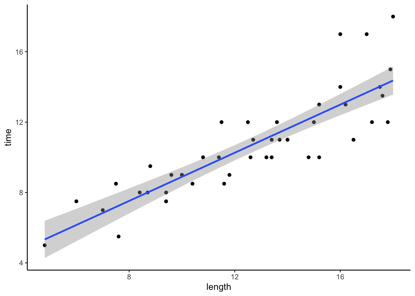

# Model the relationship
peaks_model_1 <- lm(time ~ length, data = peaks)
coef(summary(peaks_model_1))

             Estimate Std. Error   t value     Pr(>|t|)
(Intercept) 2.0481729 0.80370575  2.548411 1.438759e-02
length      0.6842739 0.06161802 11.105095 2.390128e-14

0.684 \pm 2*0.062 = (0.684 - 0.124, 0.684 + 0.124) = (0.560, 0.808)
.

confint(peaks_model_1, level = 0.95)

                2.5 %    97.5 %
(Intercept) 0.4284104 3.6679354
length      0.5600910 0.8084569

Exercise 2: Interpreting the CI

Solution

\beta_1 measures the change in the expected completion time for each additional 1 mile in length
We’re 95% confident that, for every additional mile in length, the expected completion time increases somewhere between 0.56 and 0.81 hours on average.

Exercise 3: time versus elevation

Solution

# Model the relationship
peaks_model_2 <- lm(time ~ elevation, data = peaks)
# Get confidence intervals
confint(peaks_model_2, level = 0.95)

                   2.5 %       97.5 %
(Intercept)  0.740776111 21.681976712
elevation   -0.002496112  0.002242234

Our sample data does not provide evidence of a significant association between hiking time and elevation. Why? The interval spans negative and positive values, including 0. Thus when accounting for the potential error in our sample estimate, it’s plausible that time is positively associated with elevation, negatively associated with elevation, or not associated at all!
No! Model lines with negative slopes, positive slopes, and even slopes of 0 can be drawn within these confidence bands.

ggplot(peaks, aes(y = time, x = elevation)) + 
  geom_point() + 
  geom_smooth(method = "lm")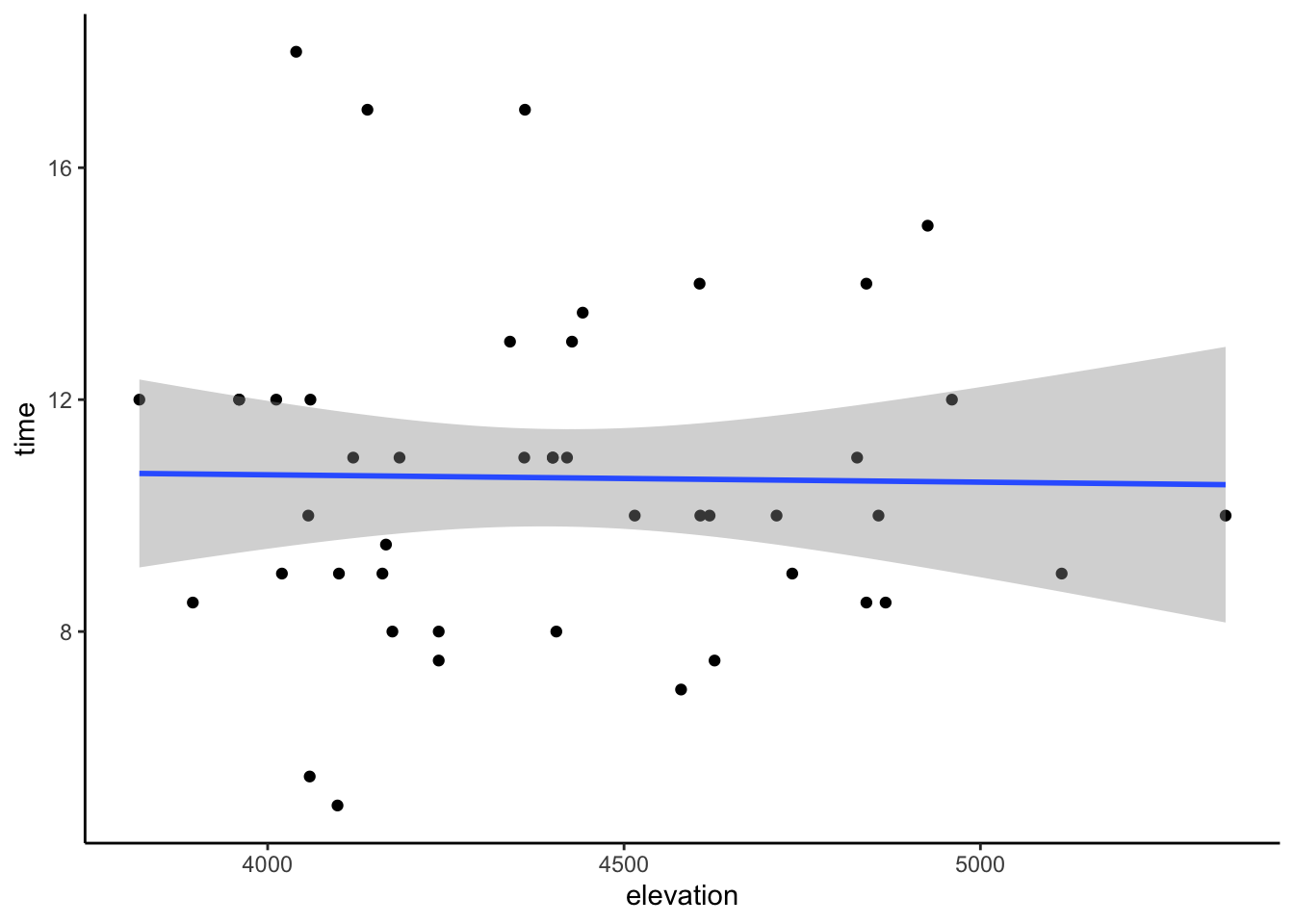

Exercise 4: time versus rating

Solution

# Visualize the relationship
ggplot(peaks, aes(y = time, x = rating)) + 
  geom_boxplot()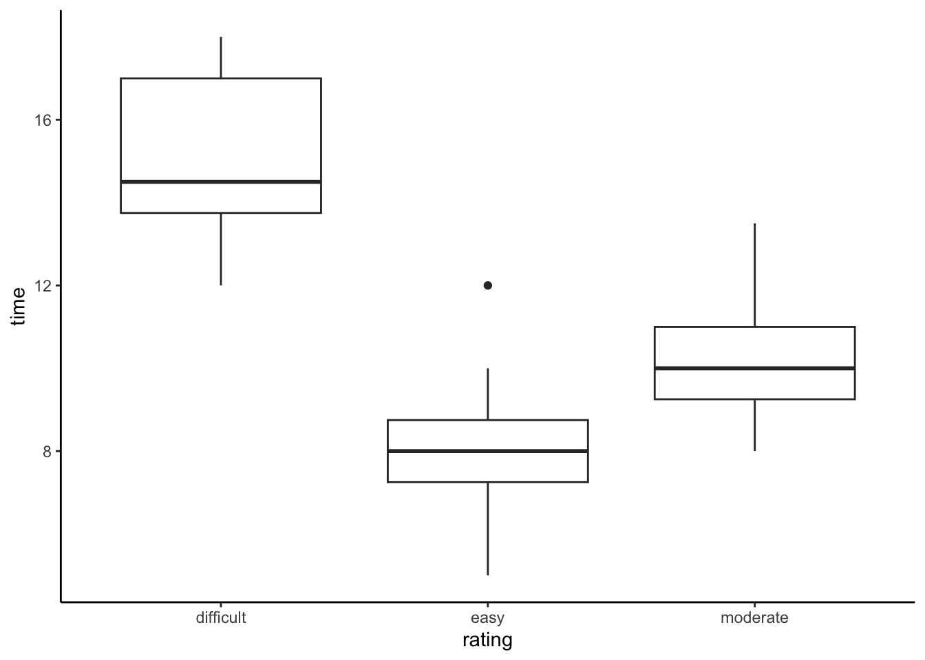

# Model the relationship
peaks_model_3 <- lm(time ~ rating, data = peaks)

# Obtain CIs for the model coefficients
confint(peaks_model_3)

                   2.5 %    97.5 %
(Intercept)    13.800649 16.199351
ratingeasy     -8.576256 -5.423744
ratingmoderate -5.921076 -3.190035

We’re 95% confident that…the average completion time of a moderate hike is between 3.19 and 5.92 hours less than that of a difficult hike
We’re 95% confident that…the average completion time of a difficult hike is between 13.8 and 16.2 hours.
Yes. The intervals for the moderate and easy rating coefficients both fall below 0, suggesting that completion times are significantly lower for moderate and easy hikes vs difficult hikes.

Exercise 5: Multiple logistic regression REVIEW

Solution

# NOTE: We'll take a sub-sample of 500 days for TEACHING PURPOSES ONLY
# In practice, we'd use all data in our sample :)
set.seed(155)
weather <- read_csv("https://mac-stat.github.io/data/weather_3_locations.csv") %>% 
  mutate(rain_tmrw = (raintomorrow == "Yes")) %>% 
  sample_n(size = 500, replace = FALSE)

# Build the sample model
weather_model_1 <- glm(rain_tmrw ~ location + humidity9am, data = weather, family = "binomial")
coef(summary(weather_model_1))

                      Estimate  Std. Error   z value     Pr(>|z|)
(Intercept)        -4.23087562 0.606988777 -6.970270 3.163334e-12
locationUluru      -0.50422768 0.413866029 -1.218336 2.230965e-01
locationWollongong  0.36535533 0.287787715  1.269531 2.042519e-01
humidity9am         0.04001737 0.008110712  4.933891 8.060742e-07

# Exponentiate the coefficients
exp(coef(weather_model_1))

       (Intercept)      locationUluru locationWollongong        humidity9am 
        0.01453965         0.60397186         1.44102595         1.04082885

rain_tmrw is binary
On a day with 0 humidity at 9am in Hobart…

The odds of rain are 0.015.
The chance of rain is 1.5% as high as the chance of no rain.

When controlling for 9am humidity levels…

the odds of rain in Uluru are 60% as high as (hence 40% lower than) the odds in Hobart.

When controlling for location…

the odds of rain increase by 4% for every additional 1-percentage point increase in 9am humidity.

Exercise 6: Inference for logistic regression

Solution

confint(weather_model_1)

                         2.5 %      97.5 %
(Intercept)        -5.45851818 -3.07261857
locationUluru      -1.35359732  0.28370308
locationWollongong -0.19609539  0.93558070
humidity9am         0.02437053  0.05626137

We do not have evidence that the chance of rain significantly differs in Uluru and Hobart when controlling for 9am humidity (i.e. when the 9am humidity is the same in both locations). 0 is in the interval!

exp(confint(weather_model_1))

                         2.5 %     97.5 %
(Intercept)        0.004259863 0.04629976
locationUluru      0.258309366 1.32803856
locationWollongong 0.821933830 2.54869305
humidity9am        1.024669914 1.05787415

We do not have evidence that the chance of rain significantly differs in Uluru and Hobart when controlling for 9am humidity. 1 is in the interval
1. An odds ratio of 1 means that the odds for the 2 scenarios are not different. For example, if odds(rain | Uluru) / odds(rain | Hobart) = 1, then the odds of rain are the same in the 2 locations.

Exercise 7: Comparing models

Solution

Yes! The interval falls above 1.

weather_model_2 <- glm(rain_tmrw ~ location + humidity9am + humidity3pm, data = weather, family = "binomial")
exp(confint(weather_model_2))

                         2.5 %     97.5 %
(Intercept)        0.000851873 0.01438824
locationUluru      0.785247399 6.16253858
locationWollongong 0.341257492 1.26391403
humidity9am        0.980908500 1.02314946
humidity3pm        1.045270255 1.09967877

No! The CI includes 1.
When controlling for location, today’s 9am humidity includes “significant” information about the chance of rain. However, it doesn’t provide significant information on top of what’s provided by 3pm humidity. It’s likely the case that 9am and 3pm humidity are multicollinear, and 3pm humidity is the stronger predictor of tomorrow’s rain.