19 The Normal model & sampling variation
Settling In
Find the qmd here: “19-sampling-normal-notes.qmd”.
Install the
gsheetlibrary by typing the following in your CONSOLE. Do NOT put this in your qmd:install.packages("gsheet")
Recap
ImportantStatistical superpowers
Thus far we’ve been using statistical models to explore and describe relationships in our sample data. We can also use them to make inferences about the broader population from which we took this sample!!!
NoteLearning goals
- Recognize the difference between a population parameter and a sample estimate.
- Review the Normal probability model, a tool we’ll need to turn information in our sample data into inferences about the broader population.
- Explore the ideas of randomness, sampling distributions, and standard error through a class experiment. (We’ll define these more formally in the next class.)
NoteAdditional resources
Required:
- Reading: Section 6 Introduction, and Section 6.6 in the STAT 155 Notes
- Video 1: exploration vs inference
- Video 2: Normal probability model
Inference
Goal: Make conclusions about the broader population that our data was drawn from.
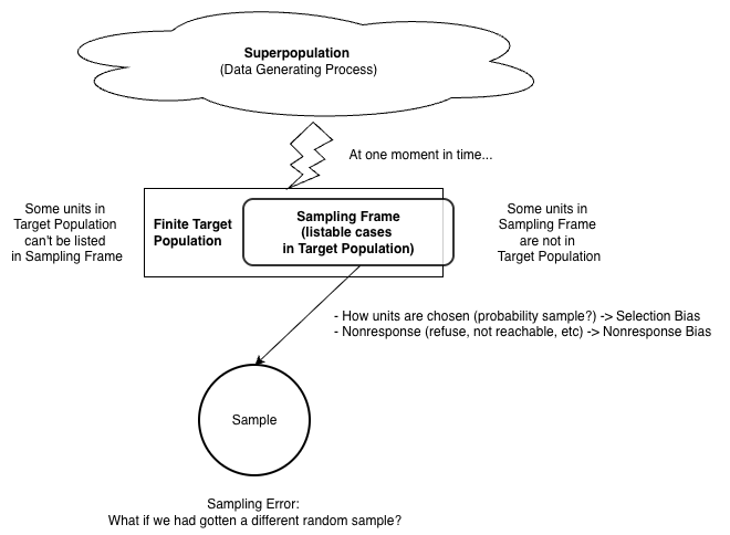
target population = the set of observations that could have ended up in our observed sample
sample = our observed data (randomly) drawn from this population, i.e. a subset of observations in the population. We want this sample to be representative of the target population.
Regression Model
Thus far in this class, we have discussed linear and logistic regression models.
Population Model: We assume this relationship between the mean outcome and explanatory variables exists in the population,
E[Y | X_1, X_2] = \beta_0 + \beta_1X_1 + \beta_2 X_2
with fixed parameters, \beta_0, \beta_1, and \beta_2, that describe the true linear relationship in the overall population that we’re interested in.
Sample Model: Assuming the population model, we use our sample data to get estimates of the parameters, \hat{\beta}_0, \hat{\beta}_1, and \hat{\beta}_2, and can write our estimated model
E[Y | X_1, X_2] = \hat{\beta}_0 + \hat{\beta}_1X_1 + \hat{\beta}_2 X_2
Probability Model
Definition: An idealistic representation of the underlying randomness in a variable, providing a sense of:
- what the values the variable can take
- the relative plausibility of those values
We go beyond specifying the mean model and use a probability model for the outcome data,
Y = \beta_0 + \beta_1X_1 + \beta_2 X_2 + \epsilon where the residuals/errors are Normal, \epsilon\sim N(0,s^2)
NOTE: The LINE assumptions we discussed include “Normal residuals/errors”. This is an assumption about the probability model.
Normal Model
One probability model is the Normal (Gaussian) model.
- This model is defined based on the center (mean = m) and spread (standard deviation = s)
X \sim N(m, s^2)
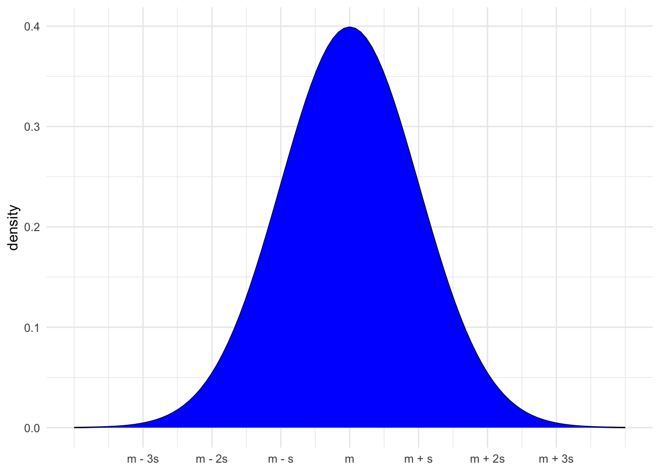
The height of the Normal curve shows the plausibility of values
- The area under the curve shows the probability of possible values.
- Area under the full curve is 1, P(-\infty < X < \infty) = 1
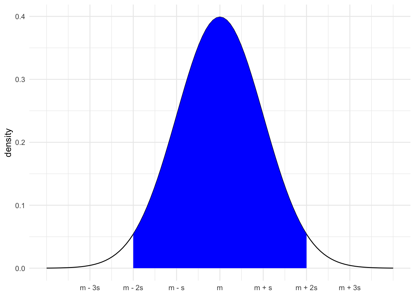
- Area under the curve within 1 sd of mean is 0.68, P(m - s < X < m + s) = 0.68

- Area under the curve within 2 sd of mean is 0.95, P(m - 2s < X < m + 2s) = 0.95
- Area under the curve within 2 sd of mean is 0.95, P(m - 3s < X < m + 3s) = 0.997

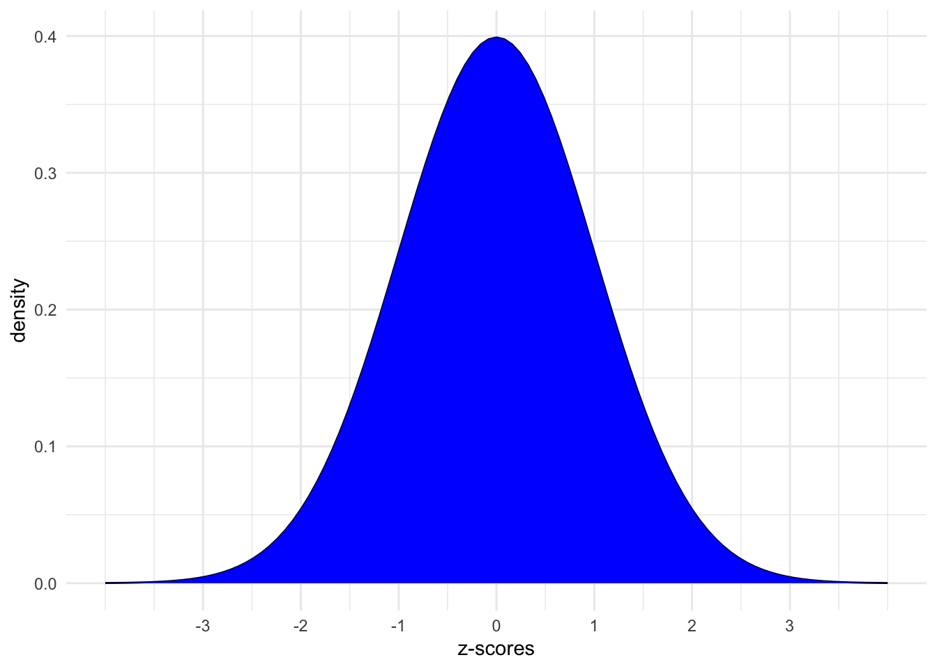
Z-scores
Definition:
\text{Z-score} = \frac{X - \text{mean}}{\text{sd}}
Meaning: how many standard deviations a value “X” is from the mean.
We can convert our values to z-scores and focus only on the standard Normal model (m = 0, s = 1),
Install new package!
We’ll need a new package today: gsheet. Install this package by typing the following in your CONSOLE. Do NOT put this in your qmd:
install.packages("gsheet")
Warm-up
Today marks a significant shift in the semester!
Thus far, we’ve focused on exploratory analysis: visualizations, numerical summaries, and models that capture the observed patterns in our sample data.
Today, we’ll move on to inference: using our data to make conclusions about the broader population from which it was taken.
Context:
The fandango dataset in the fivethirtyeight package includes information about the ratings of 143 films released in 2014-2015 across the review sites Fandango, IMDB, RottenTomatoes, and MetaCritic.
Our goal will be to model the relationship between the RottenTomatoes “Tomatometer” rating (an aggregate of official film critic scores), and the RottenTomatoes “User Rating,” which averages the ratings of anyone who uploaded their rating to the site.
# Load the data
library(fivethirtyeight)
data(fandango)

fandango <- fandango %>%
  select(film,
          userscore_rt = rottentomatoes_user,
          criticscore_rt = rottentomatoes)

# Plot the relationship
fandango %>%
  ggplot(aes(x = criticscore_rt, y = userscore_rt)) +
  geom_point() +
  geom_smooth(method = "lm", se = FALSE)

# Model the relationship
m1 <- lm(userscore_rt ~ criticscore_rt, data = fandango)
summary(m1)
POPULATION vs SAMPLE
This dataset is by no means a comprehensive collection of films and their review scores–it does not contain every film that was released from 2014-2015, nor films released outside of that date range. The review scores are also frozen in time–all of these films have almost certainly accumulated additional reviews since the data were first collected.
However, our stated goal is to make inferences about the overarching relationship between critic reviews and user reviews for all films (relatedly, we may want to use our model to make predictions about how user reviews are affected by critic reviews for films that may not even exist yet!). Can we actually make these inferences/predictions about a potentially infinite collection of films when all we have is a fairly limited subset of these?
This question points to two of the most important concepts in the field of statistical inference: populations and samples.
Statisticians have many different ways of defining a population (depending on the questions they are asking), but for the purposes of this exercise:
population = the set of all possible films and all possible review scores that have been or could be catalogued on RottenTomatoes
sample = our dataset of 146 films is a sample from this population, i.e. a subset of observations in the population.
PARAMETERS vs ESTIMATES
In order to conduct statistical inference using linear regression, we must assume that there is some true, underlying, fixed intercept and slope \beta_0 and \beta_1, that describe the true linear relationship in the overall population that we’re interested in.
For example, in modeling the relationship between UserScore and CriticScore on RottenTomatoes, the “true” underlying model we assume is:
E[UserScore \mid CriticScore] = \beta_0 + \beta_1 CriticScore
However, the “true” values of \beta_0 and \beta_1 are typically impossible to know! Knowing them would require access to our entire population of interest (in this case, the review scores for every film that has been or will be released). When we fit a regression model using the sample that we do have, we are actually obtaining estimates of those true population parameters (note the notation change of putting a \hat{ } on top of the Betas, to indicate that this is an estimate):
E[UserScore \mid CriticScore] = \hat{\beta}_0 + \hat{\beta}_1 CriticScore
In summary:
- \beta = the “true” but unknown population parameter
- \hat{\beta} = a sample estimate, i.e. an estimate of \beta calculated using our sample data
!!PRETEND!!
For the sake of this activity, let’s assume that our sample estimates, obtained above, are identical to the true population parameters. That is, assume that the “true” population model is:
E[UserScore \mid CriticScore] = \beta_0 + \beta_1 CriticScore = 32.3 + 0.52 CriticScore
🚩🚩🚩 WARNING: Be very careful not to make this assumption in other models you encounter. For this dataset, recall the specific sampling criteria that were used, which means these 146 films likely aren’t representative of the full population of films we’re interested in. This means that the estimates we obtained probably don’t match the true population parameters–they may or may not be close, but we don’t know for certain! 🚩🚩🚩
Example 1: Intuition
Below, we’ll simulate how parameter estimates are impacted by taking different samples. You’ll each take a random sample of 10 films in the dataset, and we’ll see if we can recover the presumed population parameters (i.e., the coefficient estimates we obtained from our model using all 146 films that were initially sampled).
What’s your intuition:
Do you think every student will get the same set of 10 films?
Do you think that your coefficient estimates will be the same as your neighbors’?
Example 2: Random sampling
Use the sample_n() function to take a random sample of 2 films
# Try running the following chunk A FEW TIMES
fandango %>%
  sample_n(size = 2, replace = FALSE)
Reflect:
How do your results compare to your neighbors’?
What is the role of
size = 2? HINT: Remember you can look at function documentation by running?sample_nin the console!What is the role of
replace = FALSE? HINT: Remember you can look at function documentation by running?sample_nin the console!
Example 3: Setting the seed
Now, “set the seed” to 155 and re-try your sampling.
# Try running the following FULL chunk A FEW TIMES
set.seed(155)
fandango %>%
  sample_n(size = 2, replace = FALSE)
What changed?
Example 4: Take your own sample
The underlying random number generator plays a role in the random sample we happen to get. If we set.seed(some positive integer) before taking a random sample, we’ll get the same results.
This reproducibility is important:
we get the same results every time we render our qmd
we can share our work with others & ensure they get our same answers
it wouldn’t be great if you submitted your work to, say, a journal and weren’t able to back up / confirm / reproduce your results!
Follow the chunks below to obtain and use your own unique sample.
# DON'T SKIP THIS STEP!
# Set the random number seed to your own phone number (just the numbers)
# NOTE: The point is to use a different number than other students.
# Any 7 digits of your number, that don't START with 0, are fine
set.seed(___)

# Take a sample of 10 films
my_sample <- fandango %>%
  sample_n(size = 10, replace = FALSE)
my_sample
# Plot the relationship of UserScore with CriticScore among your sample
my_sample %>%
ggplot(aes(y = userscore_rt, x = criticscore_rt)) +
geom_point() +
geom_smooth(method = "lm", se = FALSE)# Model the relationship among your sample
my_model <- lm(userscore_rt ~ criticscore_rt, data = my_sample)
coef(summary(my_model))REPORT YOUR WORK
Log your intercept and slope sample estimates in this survey.
Exercises
Exercise 1: Using the Normal model
Before getting back to the experiment, let’s practice the concepts you explored in today’s video.
First, run the following code which defines a shaded_normal() function which is specialized to this activity alone:
library(tidyverse)
shaded_normal <- function(mean, sd, a = NULL, b = NULL){
min_x <- mean - 4*sd
max_x <- mean + 4*sd
a <- max(a, min_x)
b <- min(b, max_x)
ggplot() +
scale_x_continuous(limits = c(min_x, max_x), breaks = c(mean - sd*(0:3), mean + sd*(1:3))) +
stat_function(fun = dnorm, args = list(mean = mean, sd = sd)) +
stat_function(geom = "area", fun = dnorm, args = list(mean = mean, sd = sd), xlim = c(a, b), fill = "blue") +
labs(y = "density") +
theme_minimal()
}Next, suppose that the speeds of cars on a highway, in miles per hour, can be reasonably represented by the Normal model with a mean of 55mph and a standard deviation of 5mph from car to car:
X \sim N(55, 5^2)
shaded_normal(mean = 55, sd = 5)- Provide the (approximate) range of the middle 68% of speeds, and shade in the corresponding region on your Normal curve. NOTE:
ais the lower end of the range andbis the upper end.
shaded_normal(mean = 55, sd = 5, a = ___, b = ___)- Use the 68-95-99.7 rule to estimate the probability that a car’s speed exceeds 60mph.
Your response here
# Visualize
shaded_normal(mean = 55, sd = 5, a = 60)- Which of the following is the correct range for the probability that a car’s speed exceeds 67mph? Explain your reasoning.
- less than 0.0015
- between 0.0015 and 0.025
- between 0.025 and 0.16
- greater than 0.16
Explain your reasoning here
# Visualize
shaded_normal(mean = 55, sd = 5, a = 67)Exercise 2: Z-scores
Inherently important to all of our calculations above is how many standard deviations a value “X” is from the mean.
This distance is called a Z-score and can be calculated as follows:
\text{Z-score} = \frac{X - \text{mean}}{\text{sd}}
For example (from Exercise 1), if I’m traveling 40 miles an hour, my Z-score is -3. That is, my speed is 3 standard deviations below the average speed:
(40 - 55) / 5Consider 2 other drivers. Both drivers are speeding. Who do you think is speeding more, relative to the distributions of speed in their area?
- Driver A is traveling at 60mph on the highway where speeds are N(55, 5^2) and the speed limit is 55mph.
- Driver B is traveling at 36mph on a residential road where speeds are N(30, 3^2) and the speed limit is 30mph.
Put your best guess (hypothesis) here
- Calculate the Z-scores for Drivers A and B.
# Driver A
# Driver B- Now, based on the Z-scores, who is speeding more? NOTE: The below plots might provide some insights.
# Driver A
shaded_normal(mean = 55, sd = 5) +
geom_vline(xintercept = 60) +
lims(x = c(18, 75), y = c(0, 0.15)) +
labs(title = "Driver A")
# Driver B
shaded_normal(mean = 30, sd = 3) +
geom_vline(xintercept = 36) +
lims(x = c(18, 75), y = c(0, 0.15)) +
labs(title = "Driver B")Your response here
Exercise 3: Sampling variation
Recall that we are assuming the population parameters are equal to the estimates we obtained from the model we fit using the initial sample of 146 films:
E[UserScore \mid CriticScore] = 32.3 + 0.52 CriticScore
Let’s explore how our sample estimates of these parameters varied from student to student:
# Import the experiment results
library(gsheet)
results <- gsheet2tbl('https://docs.google.com/spreadsheets/d/11OT1VnLTTJasp5BHSKulgJiCbSLiutv8mKDOfvvXZSo/edit?usp=sharing')Plot each student’s sample estimate of the model line (gray). How do these compare to the assumed population model (red)?
fandango %>%
ggplot(aes(y = userscore_rt, x = criticscore_rt)) +
geom_abline(data = results, aes(intercept = sample_intercept, slope = sample_slope, linetype=section), color = "gray") +
geom_smooth(method = "lm", color = "red", se = FALSE)Exercise 4: Sample intercepts
Let’s focus on just the sample estimates of the intercept parameter:
results %>%
ggplot(aes(x = sample_intercept)) +
geom_density() +
geom_vline(xintercept = 32.3, color = "red")Comment on the shape, center, and spread of these sample estimates and how they relate to the (assumed) population intercept (red line).
Your response here
Exercise 5: Slopes
Suppose we were to construct a density plot of the sample estimates of the criticscore_rt coefficient (i.e. the slopes).
- Intuitively, what shape do you think this plot will have?
Your response here
- Intuitively, around what value do you think this plot will be centered?
Your response here
- Check your intuition:
results %>%
ggplot(aes(x = sample_slope)) +
geom_density() +
geom_vline(xintercept = 0.52, color = "red")- Thinking back to the 68-95-99.7 rule, visually approximate the standard deviation among the sample slopes.
Your response here
Exercise 6: Standard error
You’ve likely observed that the typical or mean slope estimate is roughly equal to the (assumed) population slope parameter of 0.52:
results %>%
summarize(mean(sample_slope))Thus the standard deviation of the slope estimates measures how far we might expect an estimate to fall from the (assumed) population slope parameter.
That is, it measures the typical or standard error in our sample estimates:
results %>%
summarize(sd(sample_slope))- Recall your sample estimate of the slope. How far is it from the population slope, 0.52?
- How many standard errors does your estimate fall from the population slope? That is, what’s your Z-score?
- Reflecting upon your Z-score, do you think your sample estimate was one of the “lucky” ones, or one of the “unlucky” ones?
Your response here
Wrap-up
- Finish and study the activity!
- Project Milestone 1 (individual) due April 6
- Quiz 2 is coming up next Monday, 3/30
- Structure: Same as Quiz 1.
- Content: Will focus on the Multiple Linear Regression and Logistic Regression units, but is naturally cumulative.
- Review session: Sunday at 2:30pm in OLRI 250
Solutions
Warm Up
Example 1: Intuition
Solution
will varyExample 2: Random sampling
Solution
# Try running the following chunk A FEW TIMES
fandango %>%
sample_n(size = 2, replace = FALSE)# A tibble: 2 × 3
film userscore_rt criticscore_rt
<chr> <int> <int>
1 The Man From U.N.C.L.E. 80 68
2 Big Eyes 69 72How do your results compare to your neighbors’? They’re different!
What is the role of
size = 2? It indicates that we want to sample 2 counties.What is the role of
replace = FALSE? It indicates that we want to sample without replacement. If we sample a county, we do not “replace” it, i.e. we cannot observe it again.
Example 3: Setting the seed
Solution
The results are the same every time and for every student!
# Try running the following FULL chunk A FEW TIMES
set.seed(155)
fandango %>%
sample_n(size = 2, replace = FALSE)# A tibble: 2 × 3
film userscore_rt criticscore_rt
<chr> <int> <int>
1 Unbroken 70 51
2 Project Almanac 46 34Example 4: Take your own sample
Solution
# DON'T SKIP THIS STEP!
# Set the random number seed to the digits of your own phone number (just the numbers)
set.seed(5555)
# Take a sample of 10 films
my_sample <- fandango %>%
sample_n(size = 10, replace = FALSE)
my_sample # A tibble: 10 × 3
film userscore_rt criticscore_rt
<chr> <int> <int>
1 Inside Out 90 98
2 Insidious: Chapter 3 56 59
3 Home 65 45
4 Jurassic World 81 71
5 Project Almanac 46 34
6 Love & Mercy 87 89
7 Focus 54 57
8 Amy 91 97
9 Escobar: Paradise Lost 52 52
10 The Salt of the Earth 90 96# Plot the SAMPLE model of Y vs X among YOUR sample data
# Compare it to the actual POPULATION model (red)
my_sample %>%
ggplot(aes(y = userscore_rt, x = criticscore_rt)) +
geom_point() +
geom_smooth(method = "lm", se = FALSE) +
geom_smooth(data = fandango, method = "lm", se = FALSE, color = "red", size = 0.5)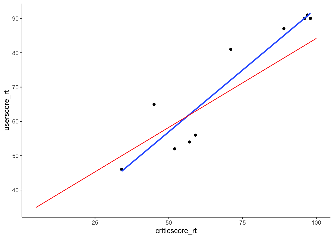
# Model the relationship among your sample
my_model <- lm(userscore_rt ~ criticscore_rt, data = my_sample)
coef(summary(my_model)) Estimate Std. Error t value Pr(>|t|)
(Intercept) 20.9883593 7.10658580 2.953367 1.833108e-02
criticscore_rt 0.7193645 0.09688257 7.425118 7.438835e-05Exercises
Exercise 1: Using the Normal model
Solution
- .
shaded_normal(mean = 55, sd = 5, a = 50, b = 60)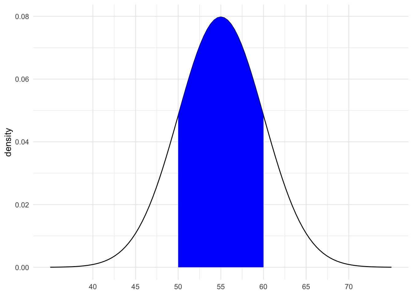
16% (32/2)
between 0.0015 and 0.025
Exercise 2: Z-scores
Solution
intuition
.
# Driver A
(60 - 55) / 5[1] 1# Driver B
(36 - 30) / 3[1] 2- B, they are 2 standard deviations above the mean (the speed limit)
Exercise 3: Sampling variation
Solution
The sample estimates vary around the population model:
# Import the experiment results
library(gsheet)
results <- gsheet2tbl('https://docs.google.com/spreadsheets/d/11OT1VnLTTJasp5BHSKulgJiCbSLiutv8mKDOfvvXZSo/edit?usp=sharing')
fandango %>%
  ggplot(aes(y = userscore_rt, x = criticscore_rt)) +
  geom_abline(data = results, aes(intercept = sample_intercept, slope = sample_slope, linetype=section), color = "gray") +
  geom_smooth(method = "lm", color = "red", se = FALSE)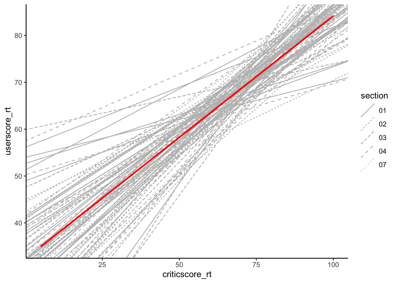
Exercise 4: Sample intercepts
Solution
The intercepts are roughly normal, centered around the intercept of the larger sample (32.3), and range from roughly 3.983 to 55.657:
results %>%
  ggplot(aes(x = sample_intercept)) +
  geom_density() +
  geom_vline(xintercept = 32.3, color = "red")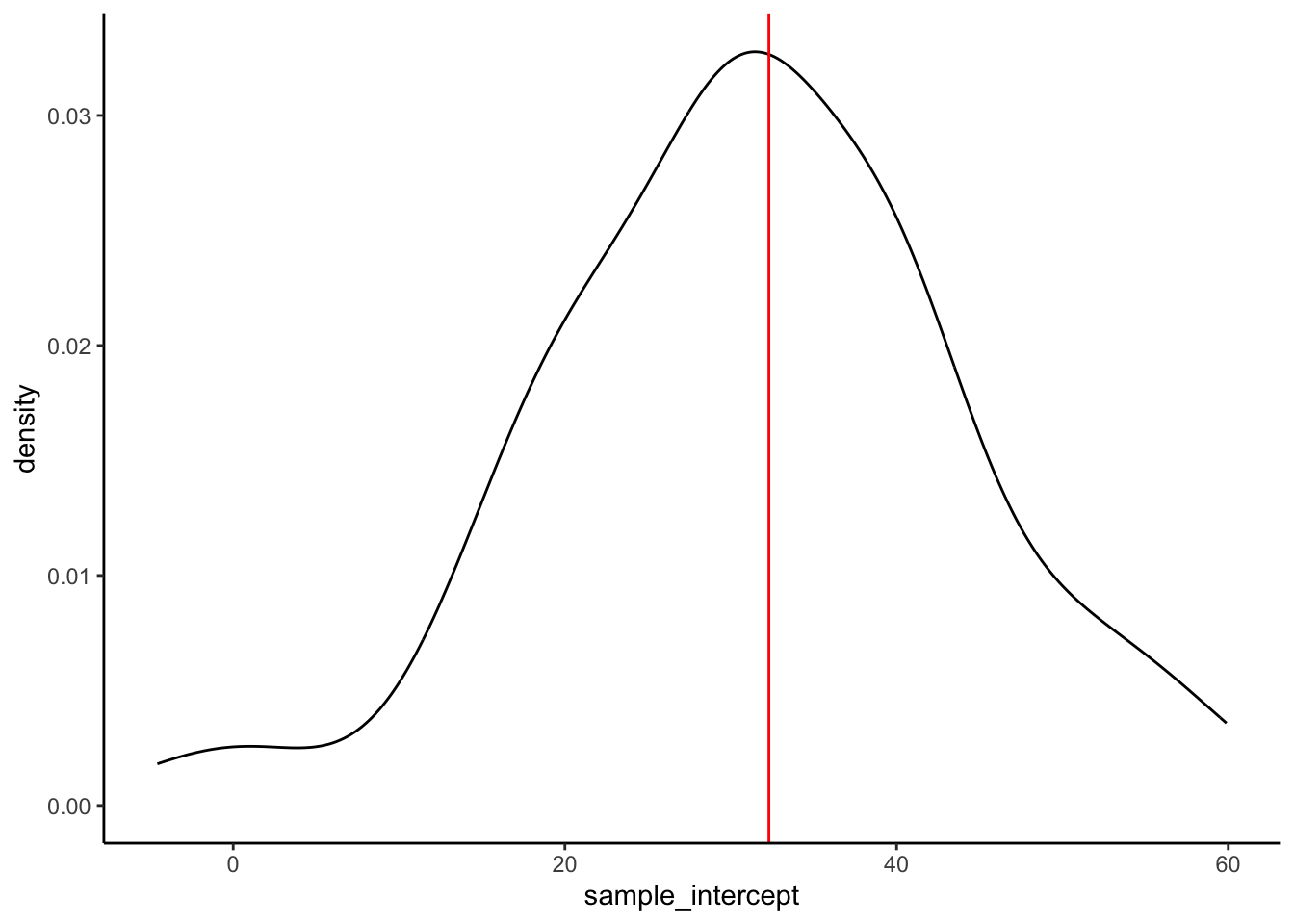
Exercise 5: Slopes
Solution
- intuition
- intuition
- Check your intuition:
results %>%
  ggplot(aes(x = sample_slope)) +
  geom_density() +
  geom_vline(xintercept = 0.52, color = "red")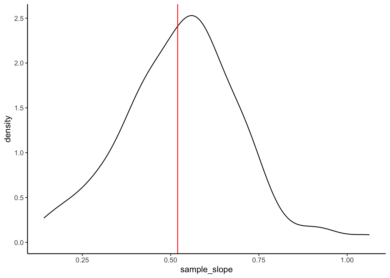
- Will vary, but should roughly be 0.17.
Exercise 6: Standard error
Solution
results %>%
summarize(mean(sample_slope))# A tibble: 1 × 1
`mean(sample_slope)`
<dbl>
1 0.530results %>%
summarize(sd(sample_slope))# A tibble: 1 × 1
`sd(sample_slope)`
<dbl>
1 0.167- For example, suppose my estimate were 0.7:
0.7 - 0.52[1] 0.18For example, suppose my estimate were 0.7. Then my Z-score is (0.7 - 0.52) / 0.17 = 1.0588235
This is somewhat subjective. But we’ll learn that if your estimate is within 2 sd of the actual slope, i.e. your Z-score is between -2 and 2, you’re pretty “lucky”.