For our 155 models, H_0: \beta_j = 0almost always.
Calculate a test statistic based on the observed sample estimate.
For our 155 models, we calculate the number of SE the observed estimate is from 0 almost always, z_{obs} =\frac{\hat{\beta}_j - \text{0}}{SE(\hat{\beta}_j)}
We figure out the sampling distribution of the test statistic.
For our 155 models, we’ll use the CLT to approximate the sampling distribution for our test statistic, Z = \frac{\hat{\beta}_j - \text{0}}{SE(\hat{\beta}_j)} \sim N(0,1)almost always
To quantify the compatibility between the observed estimate and our assumed null hypothesis H_0, we calculate the p-value:
the probability of getting a test statistic as or more extreme than observed, assuming the null hypothesis is true.
In notation, P(|Z| \geq |z_{obs}| \quad | \quad H_0\text{ is true}).
Make a decision / conclusion. We can two things. Either…
Our results are “statistically significant”.
We have enough evidence to rejectH_0 in favor of H_a
The observed data is clearly not compatible with the assumption of H_0.
NOTE: this does not mean that we “accept” H_a, we just “have evidence” for it.
Our results are not “statistically significant”.
We do not have enough evidence to reject H_0, i.e. we fail to rejectH_0.
The observed data is compatible with the assumption of H_0.
NOTE: This does not mean that we “accept” H_0, we just “don’t have enough evidence” to to reject it.
In our model summary() table, the reported test statistic (t value) and p-value (Pr(>|t|)) correspond to the following “t-test”:
H_0: \beta_j = 0
H_a: \beta_j \ne 0
The meaning or intepretation of these hypothesis depends upon the meaning of \beta_j, which itself depends upon:
whether the corresponding X predictor is quantitative or categorical
what other predictors are in the model
Why t instead of z?
In the summary() output, the p-value is calculated assuming the sampling distribution is a Student’s t model instead of a Normal model. In practice, the exact p-values will be quite similar to those from a Normal model for large enough n.
Other Hypothesis Tests
Everything is regression! Regression is everything!
In practice, people often name specific types of hypothesis tests.
Though not taught this way in AP Stat or more traditional intro courses, many of these just boil down to specific regression models.
Meaning, you already know how to do these tests!
For example:
two-sample t-test
A test for the difference between 2 population group means.
Example: Testing hypotheses about \beta_1 in the model of wage by marital status
one-sample t-test
A test for the comparison of 1 population mean to some null value.
Example: Testing hypotheses about \beta_0 in the model of wage by marital status
Warm-up
GOAL
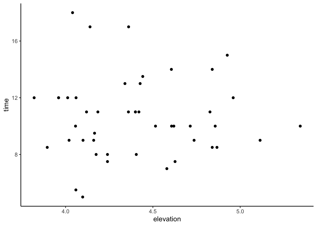
Understand the population model of hiking time (in hours) by the highest elevation of the hike (in 1000s of feet):
E(time | elevation) = \beta_0 + \beta_1 elevation
We can make inferences about this relationship using data on a sample of hikes in the peaks data:
# Load packages & datalibrary(tidyverse)peaks <-read.csv("https://mac-stat.github.io/data/high_peaks.csv") %>%mutate(elevation = elevation/1000)# Plot the relationshippeaks %>%ggplot(aes(x = elevation, y = time)) +geom_point()
# Model the relationshiphike_model <-lm(time ~ elevation, data = peaks)coef(summary(hike_model))
              Estimate Std. Error    t value  Pr(>|t|)
(Intercept) 11.2113764   5.195380  2.1579512 0.0364302
elevation   -0.1269391   1.175554 -0.1079824 0.9145006
We estimate that, for every additional 1000 feet in elevation, the expected / average hiking time decreases by 0.13 hours (~8 minutes).
We expect that this estimate might be off by / have an error of 1.18 hours per 1000 feet.
We’re 95% confident that, in the broader population of hikes, an additional 1000ft in elevation is associated with anywhere from a 2.50 hour decrease to a 2.24 hour increase in expected / average hiking time. Thus we do NOT have statistically significant evidence that hiking time is associated with elevation (a change of 0 is in this interval, hence is a plausible value).
Example 1: Starting a formal hypothesis test
H_0: hiking time is not associated with elevation H_a: hiking time is associated with elevation
Translate this to \beta notation:
H_0:
H_a:
NOTE: We will evaluate these hypotheses using a 0.05 significance level. It’s important to choose our significance level before starting our test to avoid post-hoc “tweaks” that suit our narrative.
Example 2: What would we expect under H_0?
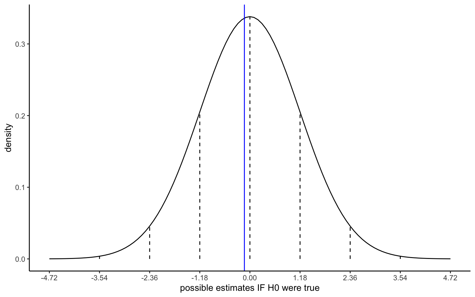
Suppose H_0 were true, i.e. \beta_1 were 0.
By the Central Limit Theorem, we’d expect the sampling distribution of possible \hat{\beta}_1 sample estimates to be Normally distributed around 0 with the standard error obtained from our model summary table:
Based on the corresponding plot below, is our sample estimate of \hat{\beta}_1 = -0.13 consistent with H_0?
# IGNORE THE SYNTAX!!!# Put OUR sample estimate hereest <--0.13# Put the corresponding standard error herese <-1.18data.frame(x =0+c(-4:4)*se) %>%mutate(y =dnorm(x, sd = se)) %>%ggplot(aes(x = x)) +stat_function(fun = dnorm, args =list(mean =0, sd = se)) +geom_segment(aes(x = x, xend = x, y =0, yend = y), linetype ="dashed") +scale_x_continuous(breaks =c(-4:4)*se) +geom_vline(xintercept = est, color ="blue") +labs(y ="density", x ="possible estimates IF H0 were true")
Example 3: Test statistic
coef(summary(hike_model))
              Estimate Std. Error    t value  Pr(>|t|)
(Intercept) 11.2113764   5.195380  2.1579512 0.0364302
elevation   -0.1269391   1.175554 -0.1079824 0.9145006
Calculate the test statistic for our hypothesis test.
Interpret the test statistic: Our sample estimate of \beta_1 is ___ [how many] standard errors ___ [above, below] the null value of ___.
So is our sample data compatible with H_0?
Example 4: p-value
Use the 68-95-99.7 Rule with the sketch from Example 2 to approximate the p-value:
less than 0.003
between 0.003 and 0.05
between 0.05 and 0.32
bigger than 0.32
Report the exact p-value from the model summary().
coef(summary(hike_model))
How can we interpret this p-value? Choose 1.
Given our sample data, it’s likely that hiking time is associated with elevation (i.e. that H_a is true). P(H_a | data) = \text{prob of $H_a$ being true given our data}
Given our sample data, it’s likely that hiking time is not associated with elevation (i.e. that H_0 is true). P(H_0 | data) = \text{prob of $H_0$ being true given our data}
If in fact there were no relationship between hiking time and elevation in the broader population of hikes (i.e. H_0 were true), it’s likely that we’d have gotten our observed decrease of hiking time with elevation “by chance”. P(data | H_0) = \text{prob of observing our data given $H_0$ is true}
So is our sample data compatible with H_0?
Example 5: Conclusion
So, at the 0.05 significance level, what’s our conclusion? Is there a statistically significant association between hiking time and elevation?
Does this conclusion agree with the one we made using the confidence interval for \beta_1, (-2.50, 2.24)?
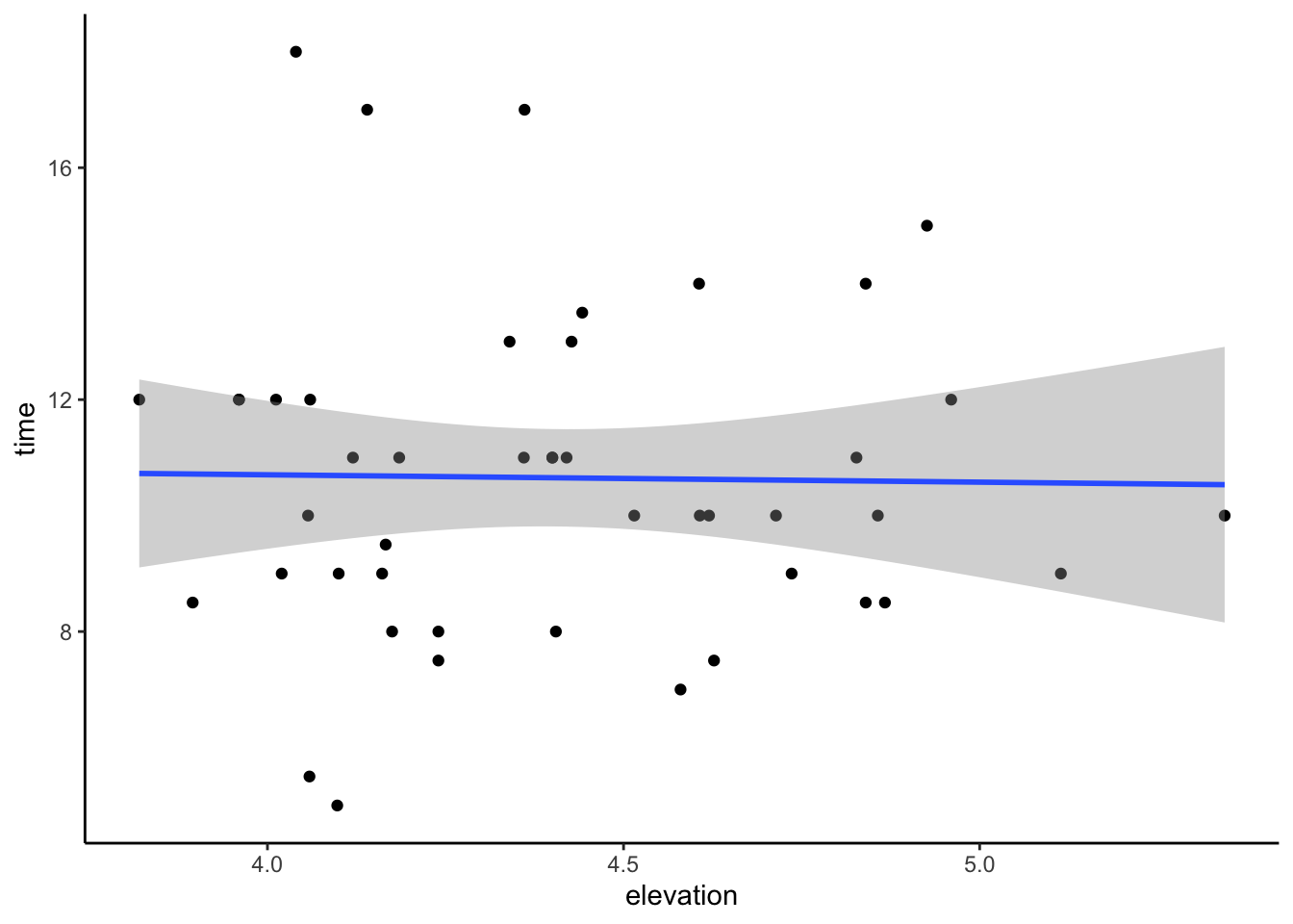
Does this conclusion agree with what we’d conclude from the confidence bands below?
peaks %>%ggplot(aes(x = elevation, y = time)) +geom_point() +geom_smooth(method ="lm")
NoteCIs, test statistics, and p-values
We’ve observed 3 equivalent approaches to determining whether or not to reject the null hypothesis that \beta equals some null value.
Assuming a 95% confidence level:
If the 95% CI for \beta does not include the null value, reject H_0!
If the p-value < 0.05, reject H_0!
If the |test statistic| > 2, reject H_0!
Example 6: tests for the intercept
H_0: \beta_0 = 0 H_a: \beta_0 \ne 0
coef(summary(hike_model))
The p-value for this test is below 0.05 (0.036). What do you conclude?
We have statistically significant evidence of a relationship between hiking time and elevation.
We have statistically significant evidence that there’s no relationship between hiking time and elevation.
We have statistically significant evidence that the average hiking time of a sea level (0 elevation) hike is non-0.
We have statistically significant evidence that the average hiking time of a sea level hike is non-0.
Research Question: Can we predict whether or not a mushroom is poisonous based on the shape of its cap?
For this exercise, we will look at data from various species of gilled mushrooms in the Agaricus and Lepiota Families. We have information on whether a mushroom is poisonous (TRUE if it is, FALSE if it’s edible) and its cap_shape (a categorical variable with 6 categories):
# Load the data & packageslibrary(tidyverse)mushrooms <-read_csv("https://Mac-STAT.github.io/data/mushrooms.csv") %>%mutate(cap_shape =relevel(as.factor(cap_shape), ref ="flat")) %>%select(poisonous, cap_shape)
Note that in the code above, we have forced the reference category for the cap_shape predictor to be flat, though its not first alphabetically:
head(mushrooms)mushrooms %>%count(cap_shape)
Part a
One of the most poisonous species of mushrooms is the Amanita phalloides or “Death Cap” mushroom, which typically has a flat cap shape when mature. Based on this anecdote, we hypothesize that species of mushrooms with flat caps in general may be more likely to be poisonous than edible.
First, let’s translate this question to an appropriate null and alternative hypothesis that we can compare with a formal hypothesis test. Remember that poisonous is a binary outcome, so we need to frame our hypotheses in terms of odds (i.e., Odds(poisonous | flat cap) = P(poisonous|flat cap)/P(edible | flat cap)).
Part b
Fit a logistic regression model to investigate if a mushroom being poisonous is associated with its cap_shape.
THINK: What’s the appropriate model – normal or logistic regression? NOTE: Remember that flat is the reference category in our table!
mushroom_mod1 <-___( )coef(mushroom_mod1)
Part c
Provide an appropriate interpretation of the estimated intercept coefficient on the odds scale. Based on this interpretation, do you believe mushrooms with flat caps are more likely to be poisonous, or more likely to be edible?
Part d
Let’s look at the full model summary:
summary(mushroom_mod1)
Report and interpret the test statistic for the intercept term (our coefficient of interest):
Part e
Report and interpret the p-value for the intercept term.
Based on this p-value and a significance level of 0.05, do we have evidence that mushrooms with flat caps are more likely to be poisonous than edible?
Exercise 2: Investigtating different cap types
Let’s continue to explore different elements of our mushroom model:
coef(summary(mushroom_mod1))
Part a
Now suppose we are interested in whether the odds of being poisonous are different for mushrooms with other cap shapes.
By hand, using the above coefficient table, calculate the odds of being poisonous for mushrooms with flat, knobbed, and conical caps. Remember: the non-exponentiated coefficients represent a difference in log-odds compared to the reference category):
odds(poisonous | flat cap) =
odds(poisonous | knobbed cap) =
odds(poisonous | conical cap) =
Part b
Relatedly, interpret the exponentiated estimates of the cap_shapeconical and cap_shapeknobbed coefficients.
Remember: these are odds ratios, comparing to flat cap mushrooms.
Part c
Based on these odds ratios, which of the 3 mushroom cap shapes would you be the most worried about eating: flat, conical, or knobbed? The least worried about eating?
Part d
Let’s get the full model summary again:
summary(mushroom_mod1)
Now report and interpret the p-values for the coefficients corresponding to cap_shapeknobbed and cap_shapeconical.
Part e
Putting this all together, if you were given a plate of mushrooms with different cap shapes and had to pick one to eat, which one would you choose? Which cap shape would you absolutely avoid at all costs? Are your decisions guided by the coefficient estimates, the p-values, or both?
Part f
Let’s look at the data a slightly different way, using a 6x2 table of counts:
Now, if you were given a plate of mushrooms with different cap shapes and had to pick one shape to eat and one to absolutely avoid, would you choose the same shapes? Why or why not?
Exercise 3
For this exercise, let’s return to the fish dataset from a previous activity.
fish <-read_csv("https://Mac-STAT.github.io/data/Mercury.csv")head(fish)
Research question: We believe the length of a fish (measured in centimeters) is causally associated with its mercury concentration (measured in parts per million [ppm]). We suspect that the river a fish is sampled from may be a confounder, since differences in the river environment may causally influence both the average length of fish (e.g. due to differences in water temperature or food availability) as well as mercury concentration (e.g. due to differences between the two rivers in mercury pollution levels).
Part a
Fit a linear regression model that can be used to answer our research question.
mod_fish1 <- ___summary(mod_fish1)
Part b
Interpret the coefficient estimate, test statistic, and p-value for the RiverWacamaw coefficient. Assume we have specified a significance level of 0.05.
Response
Part c
Suppose we now want to determine if the causal effect of fish length on mercury concentration differs according to the river from which a fish was sampled.
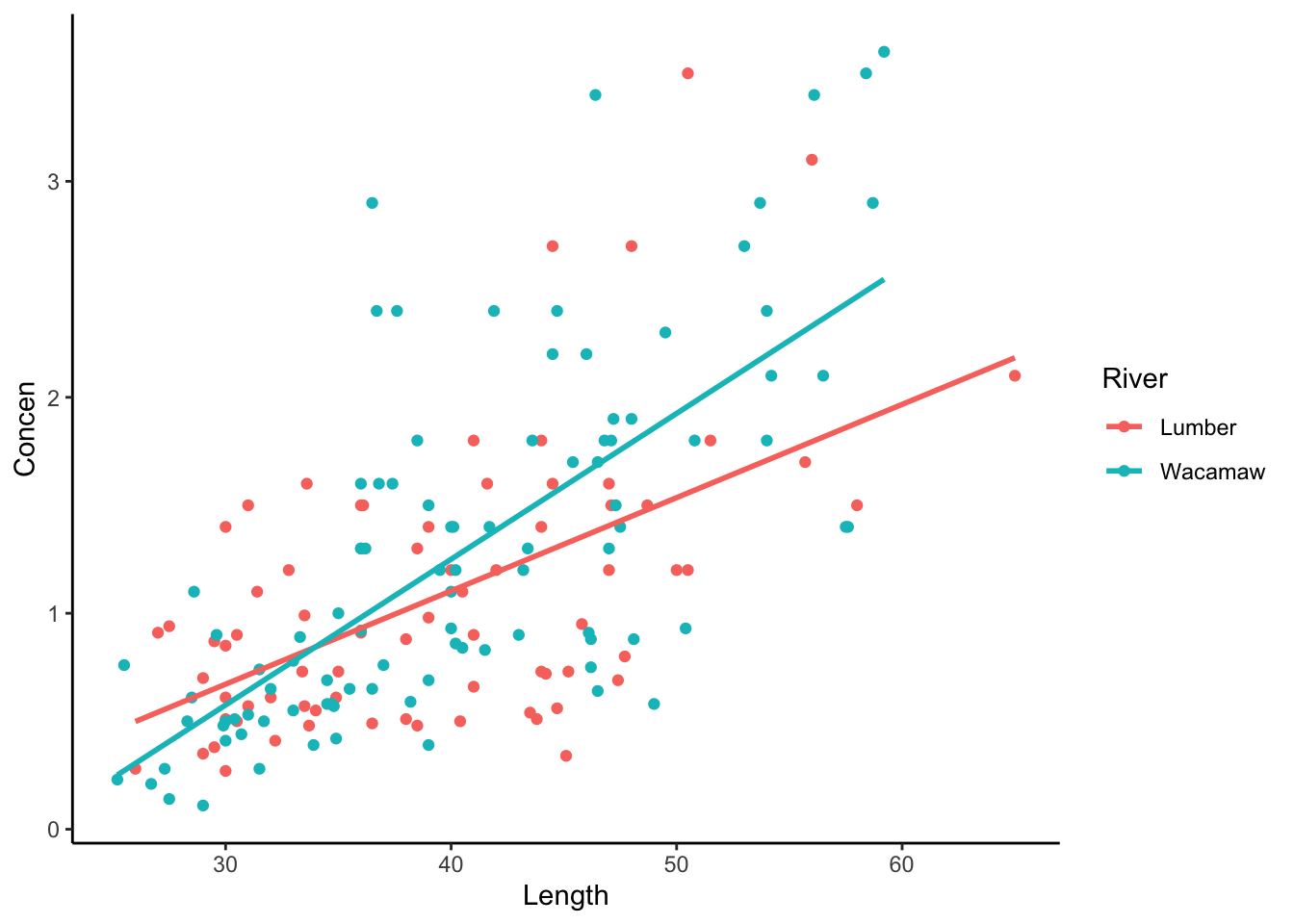
First, modify the code chunk below to visualize the 3-way relationship between the Concen, Length, and River variables.
fish %>%ggplot(aes(x = ___, y = ___, colour = ___)) +# [ADDITIONAL GGPLOT LAYER(S)]
Next, fit an appropriate linear regression model with an interaction term to investigate this question.
mod_fish2 <- ___summary(mod_fish2)
Part d
Interpret the coefficient estimate, test statistic, and p-value for the RiverWacamaw:Length interaction term in this revised model (mod_fish2). Assume we’ve set a significance level of 0.05.
Part e
Interpret the coefficient estimate, test statistic, and p-value for the RiverWacamaw coefficient in this revised model (mod_fish2). (again, you can assume we’ve set a significance level of 0.05).
Part f (CHALLENGE)
Suppose another researcher runs the same model we fit in part c above (mod_fish2), but they claim that a more appropriate alternative hypothesis should be \beta_1 < 0, (and not \beta_1 \ne 0, as is assumed by default when running a regression model). Because of this, they reported a smaller p-value for the coefficient, and claim that the Wacamaw River has a lower baseline mercury concentration (i.e., when Length = 0cm).
What is the p-value they would have reported for the RiverWacamaw coefficient in mod_fish2?
What is a potential ethical problem with the other researcher’s claim that the alternative hypothesis should be \beta_1 < 0?
Part g (CHALLENGE)
You point out to the other researcher that the intercept and RiverWacamaw coefficients are both negative, so whatever difference in mercury concentration between the two rivers your model predicts “at baseline” is not useful or meaningful–you cannot have a fish that is 0cm long, nor a mercury concentration < 0ppm.
You propose that a more appropriate model should transform the Length variable in some way to make the intercept more interpretable. Create a new variable named Length_adj with this transformation and use it to re-fit the model:
# Create a new variable# Then refit the modelmod_fish3 <-lm(Concen ~ Length_adj*River, data=fish)summary(mod_fish3)
Compare the output of this model to that of mod_fish2. What happened to the estimate, test statistic, and p-value for the RiverWacamaw coefficient? How does this affect your conclusion? How about the other researcher’s conclusion?
Wrap Up
Finish and study the activity!
PS 7 due next Monday
Check out the course schedule for other upcoming due dates (last CP coming up!).
Reminders:
Remember the important basics: complete activities, ask for help, study on a regular basis, start assignments early.
If you miss class on a project day, it’s your responsibility to communicate with your group, find out what you missed, and make equivalent contributions outside of class. If missing class on project days becomes a pattern, it will impact your project grade.
Your final project grade will reflect your individual engagement and contributions to the project. You are not expected to be perfect. Rather, you should put effort, attention, and reflection into the following areas:
communication
contributing to group discussions
including all other group members in discussion
creating a space where others felt comfortable sharing ideas and mistakes
communicating with your group outside class
report contributions
contributing to the content / analysis in the report
contributing to the writing of the report
contributing to the editing of the report
Solutions
# Load packages & datalibrary(tidyverse)peaks <-read.csv("https://mac-stat.github.io/data/high_peaks.csv") %>%mutate(elevation = elevation/1000)# Plot the relationshippeaks %>%ggplot(aes(x = elevation, y = time)) +geom_point()
# Model the relationshiphike_model <-lm(time ~ elevation, data = peaks)coef(summary(hike_model))
              Estimate Std. Error    t value  Pr(>|t|)
(Intercept) 11.2113764   5.195380  2.1579512 0.0364302
elevation   -0.1269391   1.175554 -0.1079824 0.9145006
# IGNORE THE SYNTAX!!!# Put OUR sample estimate hereest <--0.13# Put the corresponding standard error herese <-1.18data.frame(x =0+c(-4:4)*se) %>%mutate(y =dnorm(x, sd = se)) %>%ggplot(aes(x = x)) +stat_function(fun = dnorm, args =list(mean =0, sd = se)) +geom_segment(aes(x = x, xend = x, y =0, yend = y), linetype ="dashed") +scale_x_continuous(breaks =c(-4:4)*se) +geom_vline(xintercept = est, color ="blue") +labs(y ="density", x ="possible estimates IF H0 were true")
Example 3: Test statistic
Solution
.
# By hand(-0.1269-0) /1.1755
[1] -0.1079541
# This is also reported in the t value columncoef(summary(hike_model))
              Estimate Std. Error    t value  Pr(>|t|)
(Intercept) 11.2113764   5.195380  2.1579512 0.0364302
elevation   -0.1269391   1.175554 -0.1079824 0.9145006
Our sample estimate of \beta_1 is 0.108 standard errors below the null value of 0.
Yes – it’s “close to” 0 (0.108 s.e. is small).
Example 4: p-value
Solution
bigger than 0.32
Our estimate is less than 1 s.e. from 0.
0.915 (as reported in the Pr(>|t|) column)
coef(summary(hike_model))
              Estimate Std. Error    t value  Pr(>|t|)
(Intercept) 11.2113764   5.195380  2.1579512 0.0364302
elevation   -0.1269391   1.175554 -0.1079824 0.9145006
If in fact there were no relationship between hiking time and elevation in the broader population of hikes (i.e. H_0 were true), it’s likely that we’d have gotten our observed decrease of hiking time with elevation “by chance”. P(data | H_0) = \text{prob of observing our data given $H_0$ is true}
yes – there’s a high chance we would’ve gotten a sample slope this far from 0 if H_0 were true.
Example 5: Conclusion
Solution
p-value > 0.05. Thus we fail to reject H_0. We do not have statistically significant evidence of an association between hiking time and elevation.
yes
Yes, we can draw an example of a 0-slope line that falls within the bands.
Example 6: tests for the intercept
Solution
We have statistically significant evidence that the average hiking time of a sea level hike is non-0.
No. Of course a hike at any elevation will take more than 0 minutes.
The odds of a flat-capped mushroom being poisonous are 0.975:1–that is, mushrooms with flat caps are very slightly less likely to be poisonous than they are edible.
summary(mushroom_mod1)
Call:
glm(formula = poisonous ~ cap_shape, family = "binomial", data = mushrooms)

Coefficients:
                  Estimate Std. Error z value Pr(>|z|)
(Intercept)       -0.02538    0.03563  -0.712   0.4762
cap_shapebell     -2.10483    0.15677 -13.426   <2e-16 ***
cap_shapeconical  14.59145  441.37169   0.033   0.9736
cap_shapeconvex   -0.10610    0.04866  -2.180   0.0292 *
cap_shapeknobbed   0.99297    0.08557  11.604   <2e-16 ***
cap_shapesunken  -14.54069  156.04846  -0.093   0.9258
---
Signif. codes:  0 '***' 0.001 '**' 0.01 '*' 0.05 '.' 0.1 ' ' 1

(Dispersion parameter for binomial family taken to be 1)

    Null deviance: 11252  on 8123  degrees of freedom
Residual deviance: 10702  on 8118  degrees of freedom
AIC: 10714

Number of Fisher Scoring iterations: 13
The test statistic is -0.712—this means that the coefficient estimate of interest is 0.712 standard errors away from (specifically, below) the null value of 0 (note that this is on the log-odds scale).
The p-value for the intercept term is 0.4762.
Interpretation: If the null hypothesis were true (i.e., the odds of being poisonous were 1), the probability of seeing a test statistic as or more extreme than |-0.712| is 0.4762. Because the p-value is greater than our significance level of 0.05, we have no evidence to suggest that a flat-capped mushroom is more or less likely to be poisonous.
The odds that a conical-capped mushroom is poisonous are 2,172,632 times higher (!) than the odds that a flat-capped mushroom is poisonous. The odds that a knobbed-capped mushroom is poisonous are 2.699 times higher than the odds that a flat-capped mushroom is poisonous.
most worried: conical
least worried: flat
cap_shapeknobbed: Our null hypothesis is that the odds ratio between flat-capped and knob-capped mushrooms is 1 (i.e., the odds of a knob-capped mushroom being poisonous are equal to the odds of a flat-capped mushroom being poisonous). If we assume the null hypothesis is true, then the probability of seeing a test statistic as or more extreme than |11.60| is 3.91e-31. Because the p-value is far below our significance level of 0.05, we take this as strong evidence that knob-capped mushrooms are much more likely to be poisonous than flat-capped mushrooms.
cap_shapeconical: Our null hypothesis is that the odds ratio between flat-capped and cone-capped mushrooms is 1 (i.e., the odds of a cone-capped mushroom being poisonous are equal to the odds of a flat-capped mushroom being poisonous). If we assume the null hypothesis is true, then the probability of seeing a test statistic as or more extreme than |0.03| is 0.974 (i.e., we are very likely to see a test statistic more extreme than |-0.03| if in fact there were no difference between flat-capped and cone-cap mushrooms in odds of being poisonous). Because the p-value is far above our significance level of 0.05, we do not have evidence that the odds of a cone-capped mushroom being poisonous differ from the odds of a flat-capped mushroom being poisonous.
Based on the model summary output above, if you were given a plate of mushrooms with different cap shapes and had to pick one to eat, which one would you choose? Which cap shape would you absolutely avoid at all costs? Are your decisions guided by the coefficient estimates, the p-values, or both?
Answers may vary–if only considering coefficient estimates, then cone-shaped caps are most likely to be poisonous and sunken-shaped caps are most likely to be edible. But if we only look at p-values, then knob-shaped caps have the strongest evidence that they are more likely to be poisonous, and bell-shaped caps have the strongest evidence that they are more likely to be edible.
Personally, I’d stick with the sunken-shaped caps for eating. Even though our model suggests there’s no evidence to believe they are less likely to be poisonous, 0 out of 32 in the sample are poisonous, which seems like the least risky choice. However, I’d tend to avoid the knob-capped mushrooms more than the cone-capped mushrooms—even though the latter are all poisonous in the sample, there were only 4 observations, so it’s possible that due to sampling variation, the odds of being poisonous for cone-capped mushrooms is lower than that of knob-capped mushrooms (where we have many more observations).
Exercise 3
Solution
fish <-read_csv("https://Mac-STAT.github.io/data/Mercury.csv")head(fish)
mod_fish1 <-lm(Concen ~ Length + River, data=fish)summary(mod_fish1)
Call:
lm(formula = Concen ~ Length + River, data = fish)

Residuals:
     Min       1Q   Median       3Q      Max
-1.19298 -0.36849 -0.07677  0.30905  1.84773

Coefficients:
              Estimate Std. Error t value Pr(>|t|)
(Intercept)  -1.194229   0.216287  -5.521 1.26e-07 ***
Length        0.057657   0.005213  11.061  < 2e-16 ***
RiverWacamaw  0.142027   0.089496   1.587    0.114
---
Signif. codes:  0 '***' 0.001 '**' 0.01 '*' 0.05 '.' 0.1 ' ' 1

Residual standard error: 0.5779 on 168 degrees of freedom
Multiple R-squared:  0.431, Adjusted R-squared:  0.4243
F-statistic: 63.63 on 2 and 168 DF,  p-value: < 2.2e-16
coefficient: Holding fish length constant, we estimate the average mercury concentration among fish in the Wacamaw River to be 0.14ppm higher than fish in the Lumber River.
Test statistic: The estimate we observe (0.14) is 1.587 standard errors higher than the null value of a 0ppm difference in mercury concentration.
p-value: Assuming the null hypothesis is true and there is no actual difference in mercury concentration among the two fish populations (adjusting for fish length), the probability of observing a test statistic as or more extreme than |1.587| is 0.114. Because 0.114 > 0.05, we do not have sufficient evidence to reject the null hypothesis, and conclude that the average mercury concentration does not differ between the two rivers.
fish %>%ggplot(aes(x = Length, y = Concen, colour = River)) +geom_point()+geom_smooth(method="lm", se=F)
mod_fish2 <-lm(Concen ~ Length * River, data=fish)summary(mod_fish2)
Call:
lm(formula = Concen ~ Length * River, data = fish)

Residuals:
     Min       1Q   Median       3Q      Max
-1.27784 -0.35402 -0.08314  0.30650  1.94304

Coefficients:
                     Estimate Std. Error t value Pr(>|t|)
(Intercept)         -0.623875   0.325576  -1.916   0.0570 .
Length               0.043185   0.008085   5.341 2.99e-07 ***
RiverWacamaw        -0.826291   0.426529  -1.937   0.0544 .
Length:RiverWacamaw  0.024326   0.010483   2.321   0.0215 *
---
Signif. codes:  0 '***' 0.001 '**' 0.01 '*' 0.05 '.' 0.1 ' ' 1

Residual standard error: 0.5705 on 167 degrees of freedom
Multiple R-squared:  0.4488,    Adjusted R-squared:  0.4389
F-statistic: 45.33 on 3 and 167 DF,  p-value: < 2.2e-16
coefficient: First, we interpret the Length coefficient–that is, among fish in the Lumber river, we expect that a 1cm increase in length is associated with a 0.043ppm increase in mercury concentration. The interaction coefficient tells us the expected change in that relationship when considering fish in the Wacamaw River instead: we expect an additional 0.024ppm increase in mercury concentration associated with a 1cm increase in length (i.e., in the Wacamaw River, we expect mercury concentration to increase by 0.067ppm per 1cm increase in fish length).
Test statistic: The estimate we observe (0.024326) is 2.321 standard errors higher than the null value of zero.
p-value: Assuming the null hypothesis is true and there is no difference in the relationship between fish length and mercury between the 2 rivers, the probability of observing a test statistic as or more extreme than |2.321| is 0.02. Because 0.02 < 0.05, we take this as evidence to reject the null hypothesis, and conclude that the effect of fish length on mercury concentration does differ slightly between the two rivers.
coefficient: Visully, the RiverWacamaw coefficient represents the difference in the y-intercepts for the best fit lines for the Lumber and Wacamaw Rivers in the part d plot. Interpretation: Among fish that are 0cm long, average fish mercury concentrations are 0.826ppm lower in the Wacamaw River than in the Lumber River.
Test statistic: The estimate we observe (-0.826291) is 1.937 standard errors lower than the null value of 0.
p-value: Assuming the null hypothesis is true, the probability of observing a test statistic as or more extreme than |-1.937| is 0.0544. Because 0.0544 > 0.05, we do not have evidence to reject the null.
What is the p-value they would have reported for the RiverWacamaw coefficient in mod_fish2?
0.0544/2 = 0.0272 (we divide the “two-tailed” p-value in half to obtain the p-value for a “one-tailed” test)
What is a potential ethical problem with the other researcher’s claim that the alternative hypothesis should be Beta_1 < 0?
It is possible that the researchers had a particular reason or incentive to publish evidence in support of their hypothesis (some potential reasons are that scientific journals are generally less interested in publishing results, a financial conflict of interests, or favoring a pet hypothesis). They could have first looked at the results of a “two-tailed” statistical test and since the p-value is very close to the traditional significance threshold of 0.05, come up with a post-hoc rationalization to perform a hypothesis test resulting in a “statistically significant” p-value. This unethical practice is known in the field as “p-hacking.”
fish <- fish %>%mutate(Length_adj = Length -min(Length))mod_fish3 <-lm(Concen ~ Length_adj*River, data = fish)summary(mod_fish3)
Call:
lm(formula = Concen ~ Length_adj * River, data = fish)

Residuals:
     Min       1Q   Median       3Q      Max
-1.27784 -0.35402 -0.08314  0.30650  1.94304

Coefficients:
                         Estimate Std. Error t value Pr(>|t|)
(Intercept)              0.464384   0.132896   3.494 0.000609 ***
Length_adj               0.043185   0.008085   5.341 2.99e-07 ***
RiverWacamaw            -0.213287   0.176778  -1.207 0.229321
Length_adj:RiverWacamaw  0.024326   0.010483   2.321 0.021520 *
---
Signif. codes:  0 '***' 0.001 '**' 0.01 '*' 0.05 '.' 0.1 ' ' 1

Residual standard error: 0.5705 on 167 degrees of freedom
Multiple R-squared:  0.4488,    Adjusted R-squared:  0.4389
F-statistic: 45.33 on 3 and 167 DF,  p-value: < 2.2e-16
The RiverWacamaw coefficient increased (and became closer to 0). The standard error decreased, but the test statistic decreased in magnitude and the p-value increased.
What happened with this transformation is that the vertical axis got shifted so that the new “zero” was at 25.2cm (the minimum fish length in the data). At this point there is a smaller difference between the Lumber and Wacamaw River lines. However, as we saw above, there does seem to be a true modest difference in the slopes of these lines so there are larger differences between the 2 rivers at larger fish lengths.